Calendar Reporting with Excel and Power Pivot

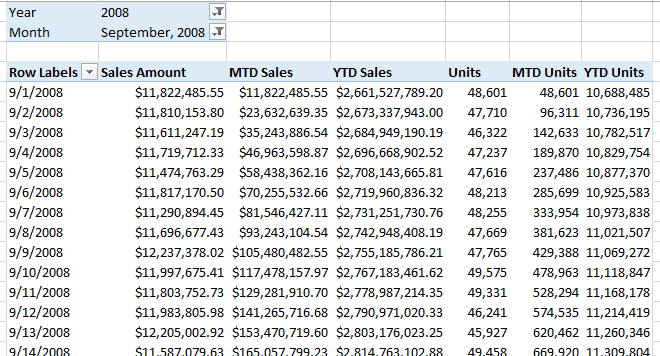
Imagine that you wanted to see a daily sales report for each day that also included month to date and year to date numbers. You could look at a large pivot table like this:

Or you could look at something that we are all a little more familiar with. A simple calendar:

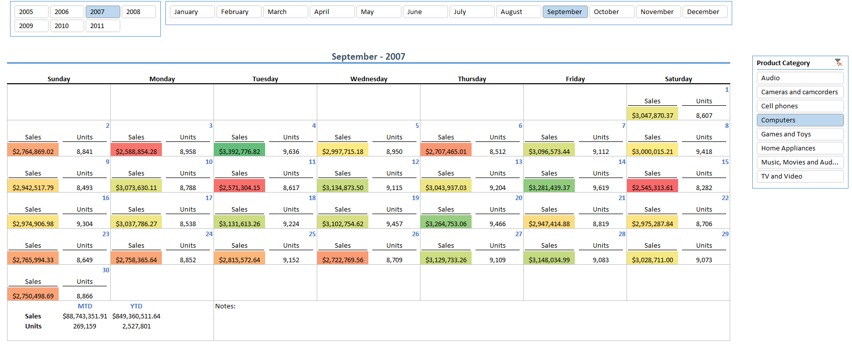
In a calendar report, metrics can be laid out naturally so that they are easy for you to find. You can do a lot more with this layout than what I have shown above. However, let’s start with how we do the basics.

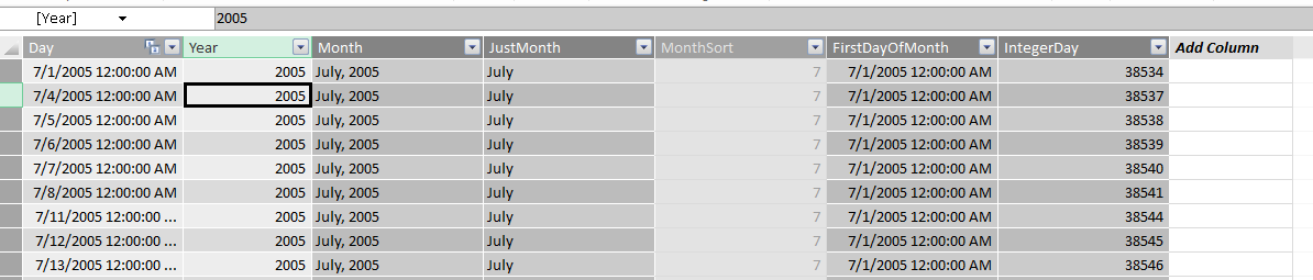
First we need to prep the date table in our Power Pivot model by making sure that we have the following columns:

We also need to add one measure to our date table called SelectedMonth. This measure will be used to figure out which month was selected in the slicers and it will drive the rest of the values in the calendar. For this measure, we need to first check that only one year and one month are selected in the slicers and if so, display what that value is. We can use the following formula that uses the HASONEVALUE function to do our check: SelectedMonth:=IF(HASONEVALUE('Date'[FirstDayOfMonth]),VALUES('Date'[FirstDayOfMonth]))

Now that we have the model prepped we can start working on Excel. Below is a blank template of a calendar.

First let’s add the slicers for Year and JustMonth:

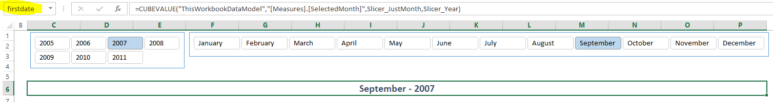
 Now that we have our slicers we can select one year and one month and then we can pick a cell to display the value of the SelectedMonth measure that we created earlier. In this case, I have chosen cell C6:

I entered the following Excel formula:

=CUBEVALUE("ThisWorkbookDataModel","[Measures].[SelectedMonth]" ,Slicer_JustMonth,Slicer_Year)

The two parameters at the end, are the named ranges for the slicers that we added for year and month.

You can then merge and format the cell to get your desired look. When you change slicer values now you should be able to see the value in the firstdate range change.

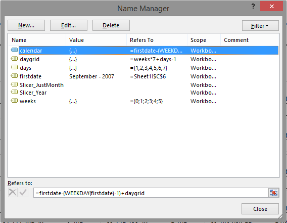
Now we need to add a few more named ranges. More detail on the formula in these ranges can be found at: https://www.advanced-excel.com/excel_calendar.html. We can add these ranges by clicking on the “Formulas” tab and clicking “Name Manager.”

Add the following:

Your name manager window should now look like this:

Now we have everything that we need to start filling in the calendar. If you go back to the template you will see that in cells A29 and A30 we have place holders for our measures. You can replace these two cells with the “CUBEMEMBER” formulas for the two measures that you want to use. In my example I used:

=CUBEMEMBER("ThisWorkbookDataModel","[Measures].[Sales Amount]","Sales")

And

=CUBEMEMBER("ThisWorkbookDataModel","[Measures].[Units]","Units")

The next step is to start filling in the days on the calendar. Before we do that, you can add any additional slicers that you want to use for filters. In my example, I added one slicer for “Product Category.”

Let’s go to the first day on the calendar. It’s sometimes helpful to pick a month that starts on a Sunday when doing this for the first time.

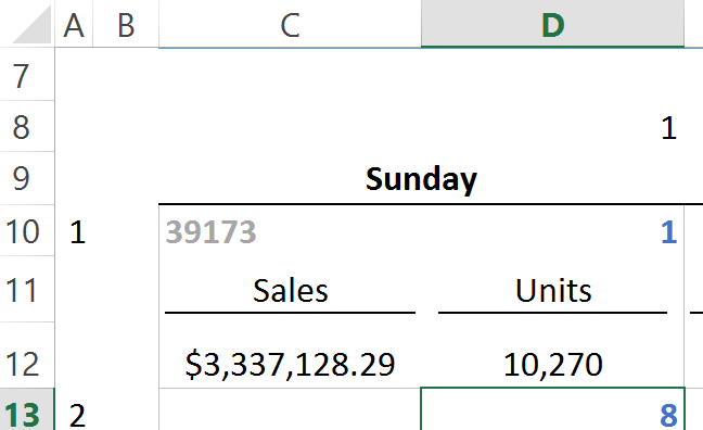
Each formula that we use from this point forward will start with: =IF(MONTH(firstdate)<>MONTH(INDEX(calendar,$A10,D$8)),"",….

We are checking to see if the date that is in the selected index is in the same month as the month that is selected in the slicers. If it is not, we return blank. Here is a breakdown of all the formulas.

Now that the first day is complete, we just need to copy all these values into the remaining days. The last step is to add any formatting and additional values that you like and we are finished.

Template and full workbook are attached at the bottom of this page. For another example, check out: https://www.powerpivotpro.com/2012/08/introducing-the-calendar-chart/

Example.zip

Comments

• Anonymous
  June 25, 2014
  Fun!

• Anonymous
  June 25, 2014
  This is great, thx for sharing

• Anonymous
  July 01, 2014
  Can you post a 2010 compatible version?

• Anonymous
  July 08, 2014
  .TY for sharing Josh!

• Anonymous
  July 30, 2014
  thanks

• Anonymous
  August 21, 2014
  On last step of calculation get #N/A error for "IntegerDay" cell (e.g. C10).  Will this not work with Excel 2010?

• Anonymous
  August 24, 2015
  OMG - Very Smart _ I like it so  much _Thank you many Thanks

• Anonymous
  August 31, 2015
  Excellent post... Thanks for sharing!

• Anonymous
  November 14, 2016
  Hi!Nice Article. I really would like to use this report on a weekly basis. But in my case I would have a slicer for planned weeks, but in my calendar I should show the next 8 weeks on actual dataThe fact table is somewhat like below where the user should Select a plannedweek from a slicer. Then the report should display all actualweeks according to the plannedweek. There is a Calendar Dimension and may be one(or two alike) week Dimensions. I have create a measure that picks up the selected week like belowSelectedWeek:=IF(HASONEVALUE('WeekCalendar'[FirstDayOfWeek]);VALUES('WeekCalendar'[FirstDayOfWeek])) But this gives me firstdayofweek for the plannedWeek not the firstday of ActualWeek. So how can I model this in powerpivot and how can I create a measure that gives me firstdayofweek of ActualWeek?|Date |PlannedWeek |AcutalWeek|Item | Amount | |-----------------------|-------------|----------|------|------------| |2014-05-12 00:00:00.000| 201419| 201420 | 10790| 8333,57| |2014-05-19 00:00:00.000| 201419| 201421 | 54| 36,74| |2014-05-26 00:00:00.000| 201419| 201422 | 642| 1072,33| |2014-06-02 00:00:00.000| 201419| 201423 | 291| 1033,7|I would like to use the same template as shown with weeks. Any example/Excel would be greatRegards Geir

• Anonymous
  November 14, 2016
  I am trying to create a report similiar to this template based on slicers and cube functions. The fact table is somewhat like below where the user should Select a plannedweek from a slicer. Then the report should display all actualweeks according to the plannedweek. There is a Calendar Dimension and may be one(or two alike) week Dimensions. I have create a measure that picks up the selected week like belowSelectedWeek:=IF(HASONEVALUE('WeekCalendar'[FirstDayOfWeek]);VALUES('WeekCalendar'[FirstDayOfWeek])) But this gives me firstdayofweek for the plannedWeek not the firstday of ActualWeek.|Date |PlannedWeek |AcutalWeek|Item | Amount | |-----------------------|-------------|----------|------|------------| |2014-05-12 00:00:00.000| 201419| 201420 | 10790| 8333,57| |2014-05-19 00:00:00.000| 201419| 201421 | 54| 36,74| |2014-05-26 00:00:00.000| 201419| 201422 | 642| 1072,33| |2014-06-02 00:00:00.000| 201419| 201423 | 291| 1033,7|Any example/Excel would be greatRegards Geir