Processing NOAA Flash Flood Guidance Data In SQL Server

**
Author:** Ed Katibah (Microsoft)
During the recent major weather event, Hurricane Sandy, NOAA published weather forecast information which would be very useful to use in the analysis of the storm. In this particular case, the data was made available as an Esri Shapefile from the following location:
http://www.srh.noaa.gov/rfcshare/ffg_download/ffg_download.php
This data was loaded into SQL Server using Safe Software’s Feature Manipulation Engine (FME).
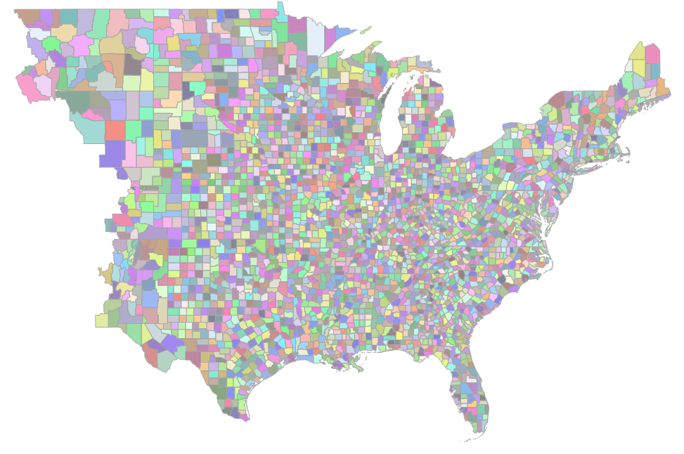
Quickly reviewing the data reveals some major points:
- The basic spatial units are counties and portions of counties
- The data covers the United States east of the Continental Divide
- Neither the state nor county names are in a form for reliable joining to other data
Here is how the spatial data appears in SQL Server Management Studio (SSMS):
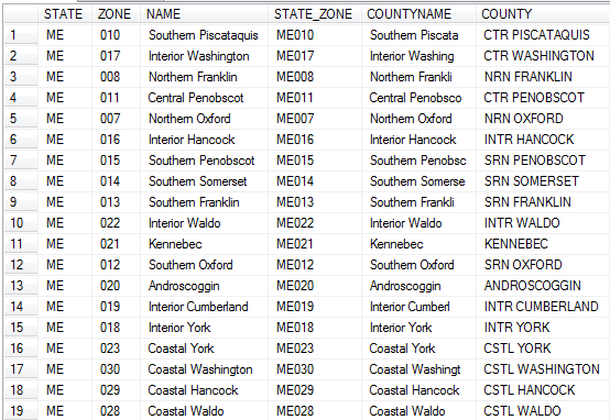
Here are the key columns which might be used to determine standardized state and county naming conventions:
Here is the full table definition:
[ID] [int] IDENTITY(1,1)
[STATE] [nvarchar](2) - State name 2-letter abbreviation
[ZONE] [nvar har](3) - Name of National Weather Service Zone
[CWA] [nvarchar](3)
[NAME] [nvarchar](72)
[STATE_ZONE] [nvarchar](5)
[TIME_ZONE] [nchar](1)
[FE_AREA] [nvarchar](2)
[LON] [float]
[LAT] [float]
[FFG_ZONE] [nvarchar](10)
[COU_CODE] [nvarchar](8)
[COU_ID] [nvarchar](10)
[COUNTYNAME] [nvarchar](16) - County name, including portion of county
[HR1] [float] - Estimated rainfall in 1 hour
[HR3] [float] - Estimated rainfall in 3 hours
[HR6] [float] - Estimated rainfall in 6 hours
[HR12] [float] - Estimated rainfall in 12 hours
[HR24] [float] - Estimated rainfall in 24 hours
[COUNTY] [nvarchar](20) - County name, including portion of county
[Geog] [geography] - Polygon representing the reporting zone
To give us an idea on what we are looking for, consider the following table. This table illustrates the use the standardized state and county identifiers – Federal Information Processing Standard Codes (FIP Codes). Columns “State” and “County” in this table are examples of FIPS Codes used to uniquely identify a state and a county within the state:
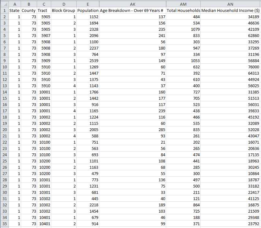
Once we have processed the NOAA data into a form which identifies states and counties using this strategy, it is easy to join to other government data which also uses this form.
Going back to the NOAA data, we have several steps to go through to get this data into a form ready for use with other data:
- Combine “portions of county” records with their logical mates to produce a single record per county
- Clip the data to represent the geographic region under analysis
- Standardize each county (and state) name so that join columns can be identified, allowing matching with other standardized data sets
To facilitate this data movement, 3 additional tables are going to be introduced:
- dbo.Counties
- dbo.CountiesFIPSCodes
- dbo.StatesFIPSCodes
These tables, along with the NOAA National Weather Service Flash Flood Guidance data (dbo.fws_ffg), make up a SQL Server database, NOAA, which is available for download on the Microsoft SkyDrive site. All of this data is derived from US Federal Government data.
Note: The following T-SQL and corresponding methodology has not been optimized. Instead, it is presented in a verbose manner which is intended to facilitate an understanding of the approach taken, in a simple, step-by-step, process.
Step 1. Establish a standardized state and county name for each NOAA zone.
The illustration below is of the 3 NOAA NWS Zone for Penobscot County, Maine showing how they are joined using the LAT and LON columns in the NOAA data. The 3 zones, Northern Penobscot, Central Penobscot and Southern Penobscot each have a latitude and longitude value in the table (LAT and LON columns). These values are for a centroid or unique location wholly within each zone. We can exploit this relationship to determine which singular county each zone lies in without resorting to parsing one of the columns which contain the zone names (and remember, counties may have the same name in different states, so we would have to add additionally logic to make sure that we have unique state/county combinations.
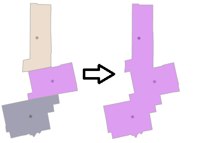
The diagram, above, illustrates how the centroid for each zone in Penobscot County, Maine is matched to a single county. This is done with spatial method, STIntersects(), a Boolean operator which evaluates to true (1) when a centroid for a given zone matches to a county polygon. Here is the SQL which is used to execute this logic:
SELECT a.STATE AS [A_STATE],
b.NAME_1 AS [B_STATE],
a.COUNTYNAME AS [A_COUNTY],
b.NAME_2 AS [B_COUNTY],
a.LAT, a.LON,
a.HR1, a.HR3, a.HR6, a.HR12, a.HR24,
a.Geog
INTO nws_ffg2
FROM nws_ffg a
JOIN counties b
ON b.geog.STIntersects(geography::Point(LAT, LON, 4326))=1
Going back to the rows with the Penobscot County, Maine zone, here is how they now appear:

The A_STATE and A_COUNTY are the original columns from the NOAA data, the B_STATE and B_COUNTY are the new, standardized, names from the Census Bureau’s Counties table.
Step 2. Get the state FIPS Code for each row
In this step we join on the standardized state name in the NOAA table (B_STATE) with the NAME column in the StatesFIPSCodes table:
SELECT A_STATE,
B_STATE,
b.STATE_FIPS_CODE,
A_COUNTY,
B_COUNTY,
a.LAT, a.LON, a.HR1, a.HR3, a.HR6, a.HR12, a.HR24,
a.Geog
INTO nws_ffg3
FROM nws_ffg2 a
JOIN statesfipscodes b
ON a.B_STATE LIKE b.NAME
Going back to the rows with the Penobscot County, Maine zone, here is how they now appear:

Note the addition of the STATE_FIPS_CODE column populated with values (23) for the state of Maine.
Step 3. Get the county FIPS Code for each row
In this step we join on the standardized state name in the NOAA table (B_STATE) with the NAME column in the StatesFIPSCodes table:
SELECT a.A_STATE,
a.B_STATE,
b.STATE_FIPS_CODE,
a.A_COUNTY,
a.B_COUNTY,
b.COUNTY_FIPS_CODE,
a.LAT, a.LON, a.HR1, a.HR3, a.HR6, a.HR12, a.HR24,
a.Geog
INTO nws_ffg4
FROM nws_ffg3 a
JOIN countiesfipscodes b
ON a.B_COUNTY LIKE REPLACE(b.NAME, ' County', '')
Going back to the rows with the Penobscot County, Maine zones, here is how they now appear:

Note the addition of the COUNTY_FIPS_CODE column populated with values (19) for Penobscot County, Maine.
Step 4. Apply a geographic filter to the NOAA data to eliminate rows not relevant to Superstorm Sandy.
To perform this step, we need a definition for the storm’s predicted path (the storm track) and a region around this storm track. For the purposes of this exercise, a distance of 400 kilometers (400,000 meters) around the storm track was chosen.
The storm track was acquired from NOAA’s National Weather Service, National Hurricane Center’s GIS Archive – Tropical Cyclone Forecast Cone site. This data is delivered in Esri shapefile format and is a 5 day forecast. There are 3 shapefiles for each date, 1 for a point data definition of the storm track, 1 for a linear definition and 1 for a polygon “probability” zone around the storm track. For our needs, the linear shapefile was chosen for the date, Oct. 30, 2012 (al182012.030_5day_lin). As with the NOAA flash flood shapefile data, the storm track data was loaded using Safe Software’s Feature Manipulation Engine (FME).
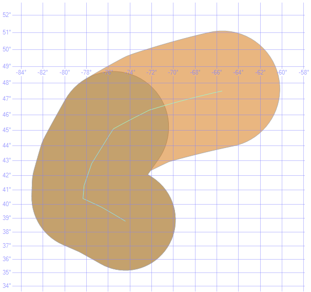
A peculiarity of the storm track linear representation is the delivery in two sections (rows). To more clearly illustrate this, here is how the storm track line appears graphically and with a 400 kilometer buffer applied:
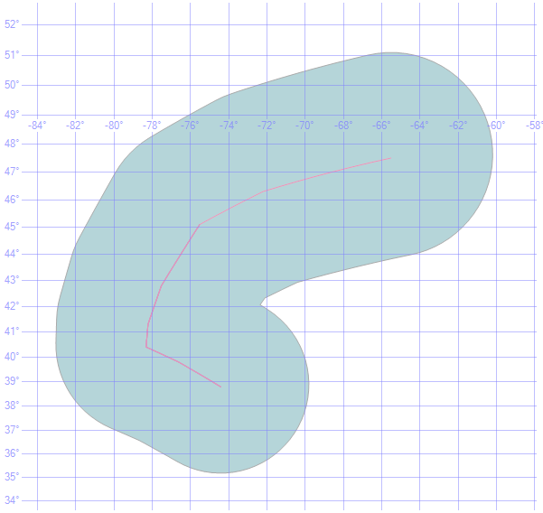
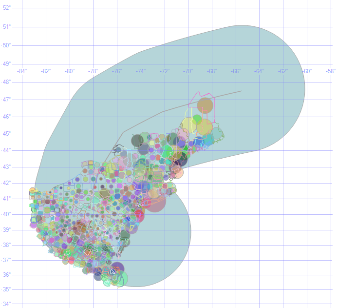
It is desirable to apply the spatial filter as a single object (1 polygon), so it is important to aggregate the storm tract into a single line and then to create a zone around that storm track. Here is how a single unified storm track appears with a 400 kilometer zone applied:
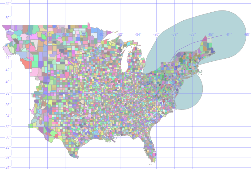
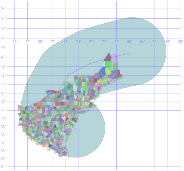
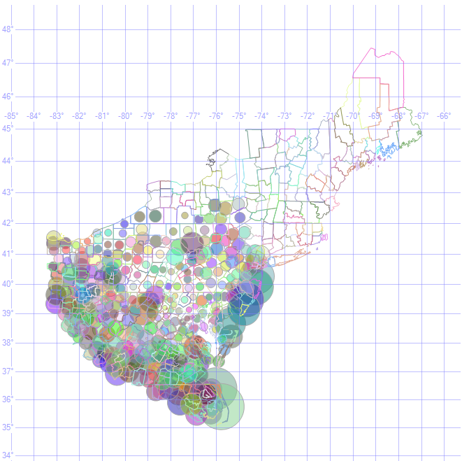
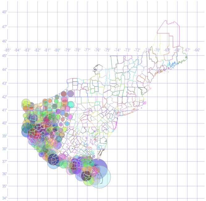
We can now take this 400 kilometer zone around the storm track and use it to clip the NOAA flash flood data. Here is the 400 kilometer zone around the storm track overlaid on the NOAA flash flood zones:
Here is the T-SQL used to do this:
DECLARE @distance INT = 400000
DECLARE @track_1 GEOGRAPHY =
(SELECT geog FROM STORM_TRACK WHERE ID = 1)
DECLARE @track_2 GEOGRAPHY =
(SELECT geog FROM STORM_TRACK WHERE ID = 2)
DECLARE @track_line GEOGRAPHY =
@track_1.STUnion(@track_2)
DECLARE @track_buffer GEOGRAPHY =
@track_line.STBuffer(@distance)
SELECT *
INTO nws_ffg5
FROM nws_ffg4
WHERE @track_buffer.STIntersects(geog)=1
Step 5. Aggregate the NOAA “Zones” into their underlying counties.
This step is a roll-up of the multiple rows which define individual zones into their underlying counties. Note the SUM function on the rainfall columns (HR1, HR3, HR6, HR12 and HR24) and the GROUP BY which rolls up to a county aggregation unit.
SELECT A_STATE, B_STATE, B_COUNTY,
STATE_FIPS_CODE, COUNTY_FIPS_CODE,
SUM(HR1) AS HR1, SUM(HR3) AS HR3, SUM(HR6) AS HR6,
SUM(HR12) AS HR12, SUM(HR24) AS HR24
INTO nws_ffg5_agg
FROM nws_ffg5 a
GROUP BY STATE_FIPS_CODE,
COUNTY_FIPS_CODE,
A_STATE,
B_STATE,
B_COUNTY
ORDER BY STATE_FIPS_CODE,
COUNTY_FIPS_CODE
Note that there are no longer any spatial columns in the asw_ffg5_agg table:

Step 6. Reattach County spatial objects to the flash flood data, now aggregated by county.
This step is necessary in order to recalculate the latitude and longitude column which will act as the “visualization” point for PowerView visualization. The true spatial columns for Centroid and Geog (the actual county polygon) are included for a sanity check on the data using the SSMS Spatial results… tab.
SELECT a.A_STATE AS State_Abbrev,
a.B_State AS State,
a.B_County AS County,
a.State_FIPS_Code AS State_FIPS,
a.County_FIPS_Code AS County_FIPS,
a.HR1, a.HR3, a.HR6, a.HR12, a.HR24,
(GEOGRAPHY::STGeomFromText((GEOMETRY::STGeomFromText(b.Geog.STAsText(), 4326).STCentroid()).STAsText(),4326)).Lat AS Latitude,
(GEOGRAPHY::STGeomFromText((GEOMETRY::STGeomFromText(b.Geog.STAsText(), 4326).STCentroid()).STAsText(),4326)).Long AS Longitude,
GEOGRAPHY::STGeomFromText((GEOMETRY::STGeomFromText(b.Geog.STAsText(), 4326).STCentroid()).STAsText(),4326) AS Centroid,
b.Geog AS Polygon
INTO nws_ffg6
FROM nws_ffg5_agg a
JOIN counties b
ON a.B_STATE LIKE b.NAME_1
AND a.B_COUNTY LIKE b.Name_2
Note*: In the SELECT list are 3 rather complicated looking spatial T-SQL statements. The core intent of these 3 statements is to obtain a single unique point within a given county. The method which performs this operation, STCentroid(), is only available for the Geometry data type. Since the county spatial column is of type Geography, we perform a "trick" by casting the Geography data to Geometry, perform the centroid operation and then recast the resulting spatial point data back to the Geography data type. This type of operation is ideal for refactoring into a user-defined function but that was beyond the scope of this exercise.
Additionally, each of these Geography --> Geometry --> Calculate Centroid --> Geography operations is compute intensive. Doing the same operation 3 times in a single query is obviously very inefficient. Need-less-to-say, in any "real" invocation of this query, this step would need to be optimized.*
Here is how our row for Penobscot County, Maine now appears:

Step 6. Visualization “sanity” checks to make sure that the processing has yield plausible results from a visual perspective.
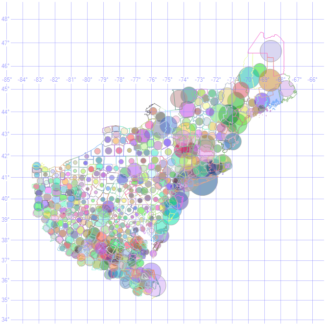
This step is a “good idea” before we refactor the flash flood table for use with PowerView-based visualization and analysis. To do this, a Dynamic SQL script was created in which the HR* columns could be used as variables and substituted easily to provide a run-through of the various flash flood potential scenarios:
DECLARE @column VARCHAR(8) = 'HR24' -- HR1, HR3, HR6, HR12, HR24 are valid values
DECLARE @radius VARCHAR(12) = '10000' -- symbol radius "scale" in meters
DECLARE @tablename VARCHAR(128) = 'nws_ffg6'
DECLARE @sql VARCHAR(2000)
SET @sql = '
SELECT GEOGRAPHY::Point([Latitude],[Longitude],4326).STBuffer(' + @column + ' * ' + @radius + ') AS POINT
FROM ' + @tablename + '
WHERE ' + @column + ' IS NOT NULL
UNION ALL
SELECT GEOGRAPHY::STGeomFromText(((GEOMETRY::STGeomFromText(Polygon.STAsText(),4326)).STBoundar
()).STAsText(),4326) AS BOUNDARY
FROM ' + @tablename +
''
EXEC(@sql)
PRINT @sql
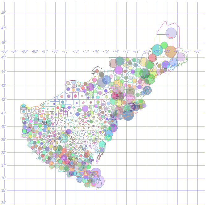
HR1

HR24
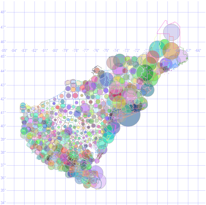
Lastly, a “mashup” of the HR3 column data is presented as a final visual check:
DECLARE @distance INT = 400000
DECLARE @track_1 GEOGRAPHY = (SELECT geog.STBuffer(@distance) FROM STORM_TRACK WHERE ID = 1) DECLARE @track_2 GEOGRAPHY = (SELECT geog.STBuffer(@distance) FROM STORM_TRACK WHERE ID = 2) DECLARE @track_buffer GEOGRAPHY = @track_1.STUnion(@track_2)
SELECT @track_buffer
UNION ALL
SELECT GEOGRAPHY::Point([Latitude],[Longitude],4326).STBuffer(HR3 * 10000) AS POINT
FROM nws_ffg6
WHERE HR3 IS NOT NULL
UNION ALL
SELECT GEOGRAPHY::STGeomFromText(((GEOMETRY::STGeomFromText(Polygon.STAsText(),4326)).STBoundary()).STAsText(),4326) AS BOUNDARY
FROM nws_ffg6
UNION ALL
SELECT Geog.STBuffer(1000) FROM STORM_TRACK -- widen storm path with a small buffer...
Step 7. Remove the spatial columns, leaving the latitude and longitude columns and create a single, unique join key for each row.
SELECT State_Abbrev,
State,
County,
State_FIPS,
County_FIPS,
HR1, HR3, HR6, HR12, HR24,
Latitude,
Longitude
INTO nws_ffg7
FROM nws_ffg6
--ALTER TABLE, ADD JOIN KEY Column and update
ALTER TABLE nws_ffg7
ADD KEYID NVARCHAR(8) NULL
UPDATE nws_ffg7
SET KEYID = CAST(State_FIPS AS VARCHAR(8)) + '_' + CAST(County_FIPS AS VARCHAR(8))
Here is how our county row looks in final form:
