SSIS: Implementing a faster distinct sort or aggregate transformation
Introduction
If you use SQL Server Integration Services to implement extract, transform and load (ETL) processes, you may have had to perform a distinct sort or an aggregation on the data passing through your data flow. In which case you will probably have use the built-in transformations and have noticed that their performance is poor.
As explained in the Microsoft documentation, these are blocking transformations. These transformations will not start yielding output until all rows have been delivered by the previous step, effectively “stalling” your data flow. As another result, memory usage requirements for your package will be high. Performance can further decline if you run out of memory as a result of these memory requirements. Buffers are going to swap to disk and performance will take another hit.

The SQL Server database engine offers some more flexibility for this sort of operation. SSIS algorithms are more generic in nature because they are designed to deal with very heterogeneous data, and so are more restrictive in their means to physically execute logical operations than the database engine.
Taking a closer look at how SQL Server manages a distinct sort or an aggregate operation at the physical level, we have two operators to choose from:
Hash Match (Aggregate)
This operator creates an in-memory hash table to store groups of rows included in the “group by” clause, along with their values. ,This may be spilled to tempdb if it runs out of execution memory. For every input row, it scans the hash table to determine whether it’s a new or an existing one, and inserts or updates values accordingly. It trades a higher requirement for processing power and execution memory for removing the requirement to first sort input rows. It can be compared to the distinct sort/aggregate steps in SSIS in terms of performance and behavior. The query optimizer will generally choose this operator if it estimates that the cost for sorting data is higher than the cost for building the hash table, which depends on the estimated number of rows, groups (or distinct values), available memory, processor speed and degree of parallelism.
Stream Aggregate
Relies on input data being sorted, either by reading from an index which is sorted on the “group by“ columns, or by having to sort it anyway (perhaps due to query hint usage or an “order by” clause). When rows are sorted by the group by clause, the algorithm looping through every row to perform calculations knows that, when the key value changes, it won’t repeat any further down the list, and thus that group calculation is complete. Performance is improved by making this a semi-blocking operation.

The distinction between the physical operators mentioned above is important because we can borrow some ideas from SQL Server and adapt these to SSIS.
One of the more obvious and simple ways to counteract the inherent issues with blocking transformations in SSIS is to perform it in the data source, when you extract data. If you are reading from a database such as SQL Server or any other major RDBMS in the market, chances are you can aggregate your data in the data source query.
Sometimes, even when reading from SQL Server, sorting at source may not be convenient. Suppose you have a complex data flow where you need to work, in parallel, both with “raw” data and aggregated results. It may not be feasible to read from the same data source twice, because of concurrency problems and increased memory usage. Using a multicast to create multiple copies of your data and then using a blocking transformation may prove to be just as bad.

Fortunately, as you may already know, SSIS supports the development of custom script tasks and transformations in VB or C#, so we can use them to create a semi-blocking transformation to eliminate duplicate rows or perform aggregations by assuming the input data is sorted. We will basically implement SQL Server’s stream aggregate physical operation in C# and use it in a data flow instead of its native, blocking counterparts.
From this point onwards, we will use a table named TEST with a single, varchar column named “COL1”. First, we want to eliminate duplicate rows and load it into a table called TEST2, with the same structure. Afterwards, we will perform a COUNT aggregation of each value and store it in a table called TEST3 (COL1 varchar(4), COL2 integer).
The base table TEST has roughly 20 million rows.
Reading data in a sorted fashion
The first step is to ensure we are reading from the source table in an ordered fashion. This can be accomplished by simply selecting SQL Statement as our source of data in the source component properties of our data flow, and then adding an “ORDER BY” clause in the select statement to retrieve all rows from TEST.
The table TEST, however, has no indexes, so the engine will always have to sort all the rows on the go, every time you run your package. In a sense, you would be just transferring some of the execution workload from SSIS to SQL Server. This may still not be a bad idea because you are avoiding a blocking transformation, reducing memory requirements, and on top of that, SQL Server sorts data faster than SSIS because it is already buffered in SS.
It goes without saying that most physical operations, if not all, are completed in a shorter time if done within SQL Server, compared to SSIS.
Let’s take a look at the execution plan for the statement responsible for extracting data in your data flow.
SELECT COL1 FROM TEST
ORDER BY COL1

A table scan, followed by a very costly, blocking sort operation. In our example, our real bottleneck will be filling the SSIS buffer with the output data from the source component, so the inherent cost in sorting data probably isn’t a real problem, but it could be. By adding an index to this table, rows will be physically stored in the key order, and thus the cost of having to sort rows every time this statement is executed will be eliminated.
CREATE CLUSTERED INDEX IDX_TEST ON TEST (COL1)
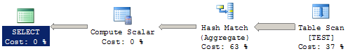
Running the same SELECT statement, even though we still have the order by clause, the physical sort operation has been eliminated:

Your source component should be something like this:

Your data flow, however, does not know that the output is sorted simply because there is an “order by” clause in your statement – you need to inform it that it is sorted. Right click your source component and select “Show advanced editor”. Click on the “input and output properties” tab and select the OLEDB Source Output. A list of properties will appear to the right of the window. Change the “Is sorted” flag to true.
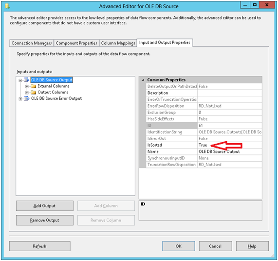
Now expand the OLEDB Source Output tree by clicking on the respective plus signal to the left of the window and then expand “Output Columns”. Each column you see here has a property called “SortKeyPosition”. Once the “Is sorted” flag is checked for the output, the “SortKeyPosition” property should match the column order listed in the “order by” clause, starting with 1. Columns not involved in the sorting should be left with the default value (zero). In our example, all we have to do here is set the “SortKeyPosition” property of the COL1 column to 1. Click “OK” when you are done.
Note that the script we are now going to implement doesn’t directly require that the input be set to “sorted”. All it really needs is that the input is in the correct order, but since other components in your data flow might require this setting, It is best to always follow the procedure above.
Creating the Script component
We are now going to create an asynchronous transformation. For more information on the basics of scripting this sort of transformation, please refer to this link.
Add a script component to the data flow and set its type to “transformation”. Connect the data source component output to the script component, right click the latter and select “Edit”.
In the “Input columns” input, select all the input columns you would like to be included in the output, both the ones in our “group by” clause and the ones we would just like to pass through. In our example, all we have to do is to select the “COL1” column.
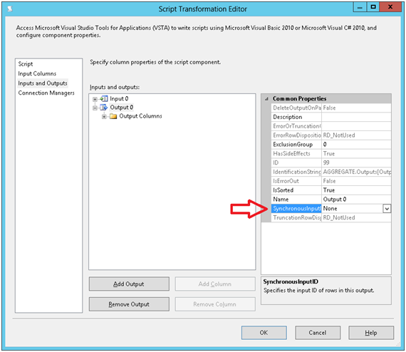
Select “inputs and outputs” in the list to the left of the window. This is where we are going to change a key setting. Select “output 0” and change its “synchronousOutputID” to “None”. Also change the “is sorted” property of the output to true and repeat the process of setting the sort key order for every column in order to match it to the input.
Now edit the script for this transformation.
The Script – DISTINCT SORT
Paste this code in the body of the class, replacing its existing content.
String previousValue;
public override  void PreExecute()
{
    base.PreExecute();
    /*
     * Add your code here
     */
}
public override  void PostExecute()
{
    base.PostExecute();
    /*
     * Add your code here
     */
}
public override  void Input0_ProcessInputRow(Input0Buffer Row)
{
    if (Row.COL1 != previousValue)
    {
        Output0Buffer.AddRow();
        Output0Buffer.COL1 = Row.COL1;
        previousValue = Row.COL1;
    }
}
The logic here is very simple: The processInputRow method receives a buffer containing a single row as a parameter. The method is executed once for every row, and reach row is processed in the sort key order.
A variable called “previousValue” is declared, initially with a null value. When the transformation starts looping through the rows and calling the ProcessInputRow method, the value of the COL1 column is compared to the previousValue variable. Whenever these values don’t match, it means a row with a new value was found and it is directed to the output buffer, and the previousValue variable is updated with this new value. Any subsequent rows with the same sort key value will match the previousValue and be discarded.
You will, of course, need to adapt this script to include your columns in it. Matching conditions must involve all the columns included in the sort key, so you’ll need a “previousValue” variable for each column. Columns that are not in the sort key and should just pass through the transformation just needs to have their value set when you call the AddRow() method of the output buffer - no other reference is required.
Comparison
The semi-blocking transformation we just implemented runs in 17 seconds on average, in my test system, and uses 50 MB.
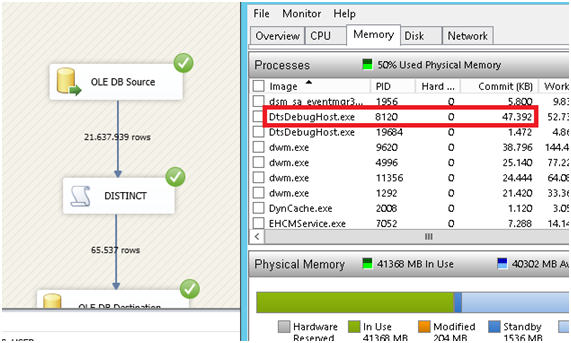
The blocking sort transformation that comes with SSIS takes 24 seconds to run and uses up to 2.5 GB memory, but it gets released as the sort transformation starts to yield its output.

Note that this does not account for all the performance improvements you may get. This is just a simple scenario where the output of the sort transformation will be immediately loaded into the destination. If there were other transformations after the distinct sort operation, they would benefit from starting their processing early on, further accelerating package execution.
An Aggregation example
This script show how the same “stream” logic can be applied to aggregations. In SQL Server, distinct sorts and aggregations are treated pretty much the same way.
String previousValue = "";
bool started = false;
int cnt = 0;
Boolean hadrows = false;

public override  void PreExecute()
{
    base.PreExecute();
    /*
     * Add your code here
     */
}
public override  void PostExecute()
{
    base.PostExecute();
}
public override  void Input0_ProcessInput(Input0Buffer Buffer)
{
    while (Buffer.NextRow())
    {
        Input0_ProcessInputRow(Buffer);
        hadrows = true;
    }
    if (hadrows && Buffer.EndOfRowset())
    {
        Output0Buffer.AddRow();
        Output0Buffer.COL1 = previousValue;
        Output0Buffer.COL2 = cnt;
    }
}
public override  void Input0_ProcessInputRow(Input0Buffer Row)
{
    if (started == false)
    {
        started = true;
        previousValue = Row.COL1;
    }
    if (Row.COL1 != previousValue)
    {
        Output0Buffer.AddRow();
        Output0Buffer.COL1 = previousValue;
        Output0Buffer.COL2 = cnt;
        previousValue = Row.COL1;
        cnt = 1;
    }
    else
    {
        cnt++;
    }
}
This time we had to make use of the ProcessInput method as well as the ProcessInputRow method. ProcessInput receives a buffer as a parameter, which is a bundle of rows, and calls ProcessInputRow for every row in the buffer. This is repeated until input buffers run out. This transformation counts the number of occurrences for each unique value in the TEST table, and its output has a new column – COL2 – of data type integer, to store the aggregation values.
The main difference here is that the very first row will always overwrite the “previousValue” variable, and the row count will start as 1. For every subsequent row with the same key, the row count is incremented by 1. Once the value changes, a new row is added with the previous value and the row count totals, and then the row count variable is reset to 1 and the “previousValue” variable is overwritten. This happens every time a new value appears.
We also have to account for the very last row, which wouldn’t be added to the output buffer because the ProcessInputRow method doesn’t know when a row is the last. If the value of the last row matches, it would simply increment the row count variable, and because the ProcessInputRow method will not be called again, the last group would be missed. So we check if the buffer has the endofrowset property set to true in the processinput method. If it is, the “current” group needs to be added to the output buffer along with its aggregation results.
This concludes our example