Power BI, Text Analytics and the Congress
Introduction
The impetus for this exercise was a video where a presenter demonstrated using IBM BigSheets to generate an interactive word cloud based upon votes in the UK parliament. The word cloud was composed of the most common words within bills voted on by the House of Lords. The presenter could click on a member of the House of Lords and the words that appeared in bills upon which that member had voted would be highlighted in the word cloud.
Nifty. So, we decided to attempt the same thing using Power BI in order to discover if we could use the same technique to gain insights into the operations of the United States Congress.
This article is split into three main sections, first an overview of the exercise’s results, second, a methodology of how we went about the exercise along with some of the key learnings and third, a detailed “how to” section. If you would like a copy of the final Power BI Designer Preview file, we have posted it here for download: https://drive.google.com/file/d/0B-sXUrtMF2h7b0JDNmVncXBQNjg.
Overview
As stated, our goal was to recreate a demonstration where the votes on bills of the members of the United Kingdom’s House of Lords were analyzed such that a word cloud was created from the text of those bills and a user could interactively select a member and the corresponding words contained in the bills that member voted upon were highlighted in the word cloud. For our project, we chose to use the United States Congress and chose to work with Microsoft’s Power BI tools.
After downloading the necessary data, we decided to use the congressional years of President Barak Obama’s presidency as our cohort. This included congressional sessional sessions 110 – 114. Unfortunately, the database we acquired only had bills passed in sessions up to and including session 112. Thus, we revised our cohort to just sessions 110 – 112. In addition, the database contained only the titles of the bills, not their full text. Finally, Power BI currently lacks a word cloud visualization and thus we decided to use a tree map visualization instead.
Below is the end result:

One can clearly see the most prominent words are “amend”, “purposes” and “bill”, followed by “act”, “states” and “united”, followed by “provide”, “code”, “certain” and “national” followed by “title”, “duty”, “federal”, “health” and “program”. As an aside, the words “responsible”, “frugal” and “compassionate”; or any of their synonyms, did not make the list of top words…
However, as we select a particular legislator, in this case Brian Schatz, a Democratic Senator from Hawaii, the tree map changes drastically to only include words that are contained in bills’ titles that Senator Brian Schatz voted upon.

A bit of investigation indicates that Senator Brian Schatz was seated on December 26th, 2012 during the waning days of the 112 session of Congress no doubt. This appointment came after the death of his predecessor, Senator Daniel Inouye.
But, the real question is, can any insights be gained. Certainly. Below are series of images showing then Senator Barak Obama’s voting record in Congress during session 110, the only session with Barak Obama contained in this cohort.
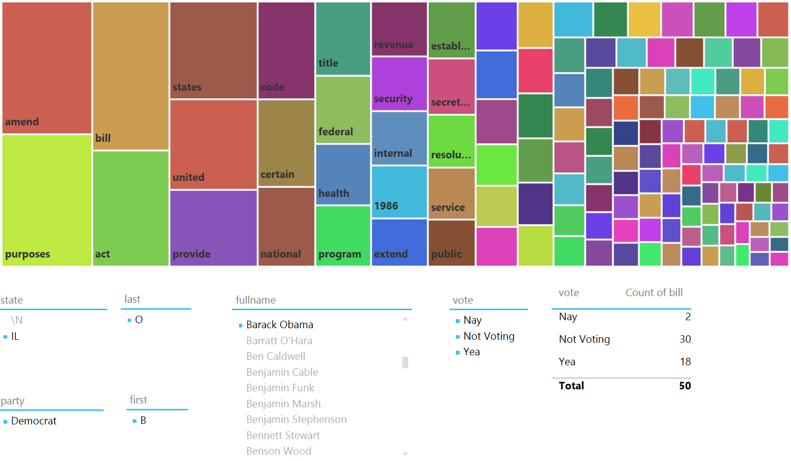
Above, we can see that then Senator Barack Obama only voted 50 times on the actual passage of bills, this puts him in the bottom 2% among all legislators in the database for number of votes cast on the passage of bills. In addition, it may be illustrative that he voted a third more times “Not Voting” than his votes for “Nay” and “Yea” combined. If we reference our first picture with all legislator votes included, this is clearly NOT typical as “Not Voting” represents just over 5% of the votes cast by legislators in the aggregate during sessions 110, 111 and 112. Therefore, with then Senator Barack Obama’s record of voting “Not Voting” 60% of the time, he was 12 times more likely to vote “Not Voting” than the average Congressional member.
Digging deeper into his “Nay” votes:

We can see he voted against the authorization of foreign intelligence and stem cell research. Switching to “Yea” votes:

We can see some words that a community organization might care deeply about, “service”, "public”, “improve”, “social” coming to the fore. Finally, if we look at “Not Voting”: 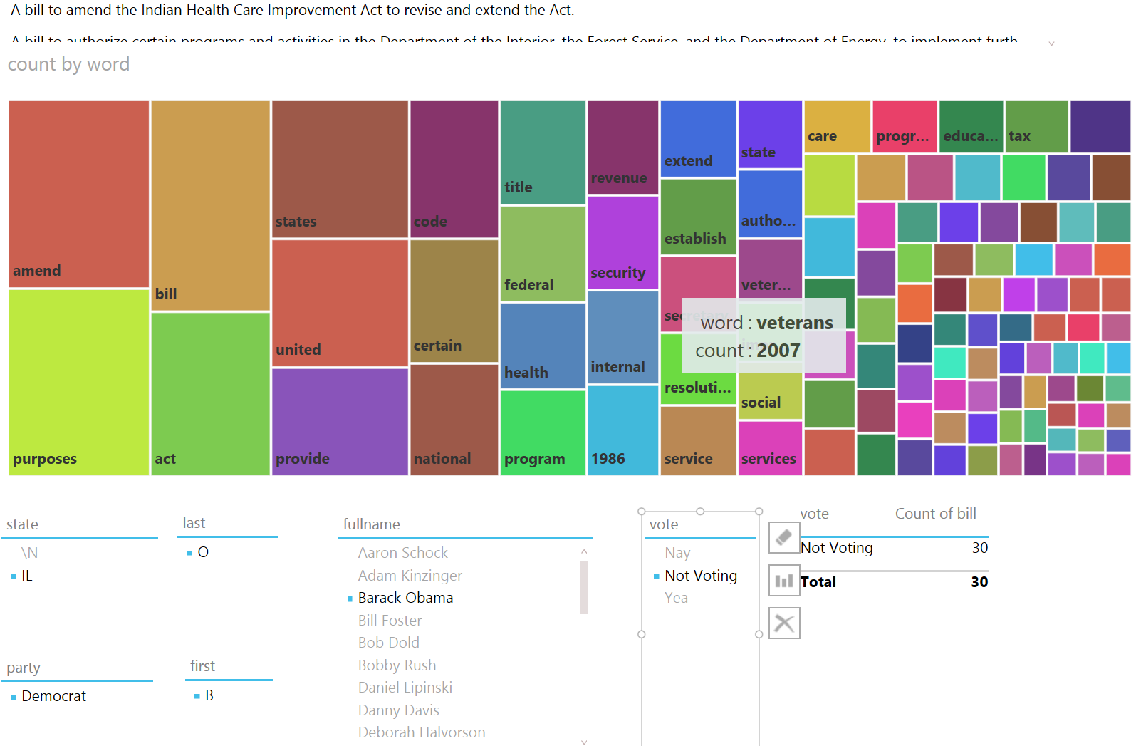
The words that jump out are “veterans”, “education” and “tax”. And, perhaps surprisingly, not voting on an Indian Health Care Improvement Act.
In general, this project serves as a model for many types of scenarios that individuals and businesses wish to better understand and derive insights from. This model is of an actor deciding upon an outcome based upon some influencer. In this case the actor is a legislator, the outcome is a vote and the influencer is a piece of legislation. However, the same basic model applies to a consumer making a buying decision based on an advertisement. In fact, the model of actor, outcome, influencer can be applied to many situations. While this project example is historical, rather than predictive, the same basic processes can be used to provide predictive metrics. For examples, we recommend checking out the source of the data used in this exercise, at www.govtrack.us, specifically their analytics prognosis page, https://www.govtrack.us/about/analysis#prognosis
Leaving you with one final visualization, while Power BI does not have a word cloud visualization, we did generate one that contained all of the top 312 words contained in the cohort. For your enjoyment.
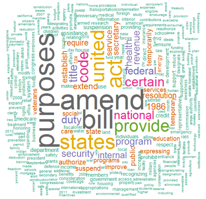
In all honesty, we was rather surprised that the top three words weren’t “spend”, “drunken”, “sailors”…
Methodology
This section provides a general summary regarding how we proceeded with this project and some of the key learnings that came out of the process.
The first question that needed to be answered was whether or not it was even possible to achieve the result that we was looking for with the given toolset, in this case Power BI. Therefore, we decided to build a simple prototype in order to prove that we was not wasting our time. we created the following files with the following data:
We imported these into Excel 2013 via Power Query and wired up our tables:

I then created a very simple Power View report with the people as a slicer and the words and their counts as a bar graph:
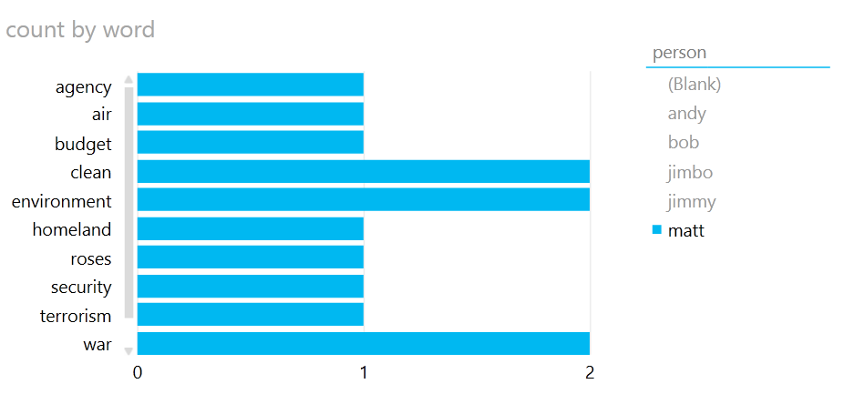
And…big bucket of fail. As can be seen above, even though “matt” is selected and “matt” only voted on one bill, all of the words from all of the bills are being displayed. Hmm. Not what we had imagined.
However, on a hunch, we attempted the exact same exercise in Power BI Designer Preview and…SUCCESS!
This led to the first revelation, Power BI Designer Preview appears to be a lot smarter about transitive relationships than PowerPivot in Excel 2013. In case we lost you there, according to Bing:
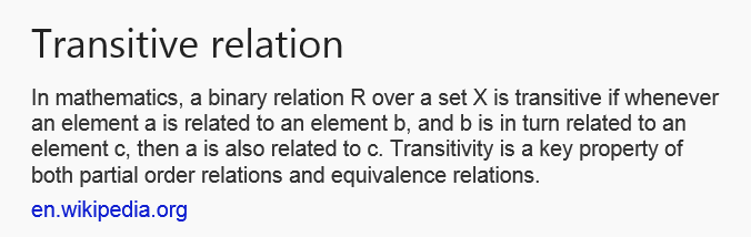
In other words, if A is related to B and B is related to C, then A is related to C. Now, if you refer back to the relationship diagram, it is a bit more complicated than A, B, C, but somehow Power BI Designer Preview is able to follow the relationships such that when we click on a person, our bar graph changes to only show the words contained in the bills that person voted on. Very nifty and exactly what we was going for.
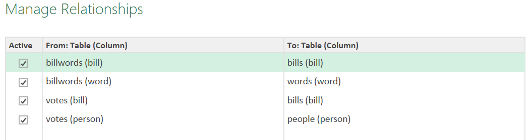
Another revelation that was related to this was that Power BI Designer Preview is also a lot smarter about figuring out relationships automatically. When we imported the exact same files in the exact same what, Power BI Designer Preview formed the following relationships without me lifting a figure:
Building this prototype was a valuable exercise. First, it confirmed that we should be able to accomplish our goal. Second, it identified the toolset that would be required to accomplish that goal, in this case Power BI Designer Preview. Third, it confirmed the viability of the core data model that we would emulate when doing our production analysis.
Armed with the knowledge that we had a solid model and toolset. we proceeded to start our data collection activities. First stop was Bing and a search for “United States Congress”. The first two results were for www.house.gov and www.senate.gov.
Unfortunately, a quick perusal of the sites left me in almost total despair. First, the sites were entirely different. Second, while the information we was seeking seemed to be on the sites, the organization and format of the information was abysmal and almost completely unusable. we briefly contemplated building a web crawler that we could use to extract the necessary information from the sites. However, after a series of dead ends and wracking our brain, we stumbled upon a fantastic site, www.govtrack.us. The organization behind this site, Civic Impulse, LLC apparently scrapes a variety of official government websites daily and extracts that information into a normalized database that they make freely available for reuse. Salvation!
Govtrack.us has a plethora of files, including the full text and votes of nearly every bill ever entered into the US House and Senate, available via rsync or web download. The data is available in a variety of friendly formats, including JSON, XML and raw text. we fired up rsync and started downloading the raw data. However, as we browsed the site, we stumbled upon a file in the “db” directory off of the root called database.sql.gz. This was almost too good to be true, could it really be a normalized SQL database that we could download and use? we downloaded the file and unpacked it. The resulting file, database.sql was almost 1.5 GB in size. A quick perusal of the file determined that it was a our SQL dump file and seemed to contain all of the SQL commands necessary to recreate the database with all of its data.
Downloaded our SQL from Oracle. Created a new schema called “govtrack” and imported the database.sql file, which imported flawlessly the first time; much to our surprise we might add. A few SELECT statements later and we confirmed that the database held everything that we needed to complete our exercise. we did have to make one small concession. The database held all of the bills’ titles but not their full text. we weighed the cost/benefit of using just the titles versus the full text and determined that for a first pass, just the titles would be good enough. Given the success thus far, we am currently deciding whether or not to revisit the project and utilize the full text of the bills. Stay tuned.
This brings me to another revelation. It is well established that data collection, data understanding and data preparation activities generally consume about 70% of any data science project. Automation can take this down to maybe 50%. Thus, particularly for external data sources, the value of third-party data aggregators is tremendous. Had we been forced to collect, organize and cleanse all of the raw data from government websites, this project would have potentially taken me weeks, months or even years to complete. Instead, we was able to complete this project in a total of about 16 hours of actual work. This included all of our prototyping, discovery, tools installation, data collection, modeling, analysis and deployment.
Once we had the data, we was able to use our SQL and R skills to manipulate the data into almost the exact same CSV files that we created in our prototype. The only significant difference was that we added a unique ID column to the “people.csv” file for forming the relationships between the other tables. we also ended up adding a “billtitle.csv” file in order to provide the full title of each bill for display purposes in our reports and dashboards and a “people_roles.csv” file for providing additional information about the people, including state, role such as Representative or Senator and party affiliation.
One last item to note is that while we was able to greatly reduce our data collection, data understanding and data preparation times through the use of the govtrack.us database, we still spent a significant proportion of our time on data understanding and data preparation. There were a number of nuances to the govtrack.us database that we needed to understand in order to get the data correct. For example, we did not immediately realize that the same bill potentially has many different titles and gets voted on potentially many times as it works its way through the system. Thus we needed to weed out the extraneous titles and votes and get to only the “official” titles and votes for when the bill was actually voted upon for passage. In addition, we had to construct a unique identifier for each bill as the database did not have one. You can read more about these challenges in the “How To” section.
How To
The first step is to make sure that you have all of the tools necessary to complete the exercise. This includes an installation of Oracle our SQL, RStudio or R, Power BI Preview tenant and an application for unpacking gzip (.gz) files.
Once those tools are installed, download the database.sql.gz file from https://www.govtrack.us/data/db/. Unpack this file to database.sql.
From our SQL Workbench, create a new schema called “govtrack”. Choose the govtrack schema as the default schema by right-clicking it and choosing “Set as Default Schema”. Choose “File” | “Run SQL Script” from the menu and choose the database.sql file. Make sure to select the “govtrack” schema and choose OK. Wait. IMPORTANT, make sure that you do NOT choose “Open SQL Script”, otherwise you will be waiting forever and then still have to execute the thing.
Once loaded, the following tables are contained within the database:
- billstatus
- billtitles
- billusc
- committees
- people
- people_committees
- people_roles
- people_votes
- votes
Create two directories
- C:\temp\govtrack
- C:\temp\govtrack\text
The next steps basically create all of the CSV files that you will need to import via Power Query into your data model in Power BI Designer Preview. Could you connect to your our SQL database directly from Power BI Designer Preview, yes you could and if you want to do that, go right ahead. The only ones that will potentially cause problems are billwords.csv and words.csv but we imagine someone can come up with a better solution than what we have below to better automate the process. Give it a try.
To generate the list of bills, use the following SQL query. Note that with this and other queries, we was still under the delusion that the database contained sessions 113 and 114, which our version did not. Also note the CONCAT used to combine the bill’s session, type and number into a single identifier. This is important as this serves as the unique key for a bill. In addition, note the titletype=’official’ portion of the WHERE clause. This is important as a bill may have multiple titles and all are tracked within the database. Finally, you may wish to change the LINES TERMINATED clause the ‘\n’ if you are on a *nix system instead of Windows.
SELECT "bill"  FROM govtrack.billtitles
UNION
SELECT CONCAT(session,type,number) as bill FROM govtrack.billtitles
WHERE (session=110 or session=111 or session=112 or session=113 or session=114)
AND titletype='official'
INTO OUTFILE '/temp/govtrack/bills.csv'
FIELDS TERMINATED BY  ','
ENCLOSED BY  '"'
LINES TERMINATED BY  '\r\n'
;
To generate a list of people, use the following SQL query. Note that including middlename in your CONCAT is a bad idea as it effectively gives everyone with a middlename of NULL a fullname of NULL, which is really not desirable.
SELECT "id","fullname" FROM  govtrack.people
UNION
SELECT id,CONCAT(firstname, ' ', lastname) AS  fullname FROM  govtrack.people
INTO OUTFILE '/temp/govtrack/people.csv'
FIELDS TERMINATED BY  ','
ENCLOSED BY  '"'
LINES TERMINATED BY  '\r\n'
;
To generate a list of people roles, use the following SQL query. This is not absolutely essential to getting to the end result, but makes it nicer to zero in on particular individuals and groups. And, yes, you could include this in your people.csv if you want, we was following our prototype model and didn’t think to include this until later as we experimented with the reporting and dashboarding.
SELECT 'personid','type','party','state'
FROM govtrack.people_roles
UNION
SELECT personid,type,party,state
FROM govtrack.people_roles
INTO OUTFILE '/temp/govtrack/people_roles.csv'
FIELDS TERMINATED BY  ','
ENCLOSED BY  '"'
LINES TERMINATED BY  '\r\n'
;
To generate a list of votes, use the following SQL query. This is really abysmal SQL for a JOIN operation between people_votes and votes. Essentially, you only want the people_votes for the selected votes, which should only include the cohort sessions of 110 – 114 AND also only include votes that contain the phrase “On Passage” as this denotes the final vote on the bill for passage versus all of the “sausage making” that occurs while the bill slowly makes its way through the legislative process.
SELECT "personid","vote","bill"
FROM govtrack.people
UNION
SELECT people_votes.personid,people_votes.displayas,
CONCAT(votes.billsession,votes.billtype,votes.billnumber) as  bill
FROM govtrack.people_votes, govtrack.votes
WHERE votes.id = people_votes.voteid
AND (votes.billsession=110 or votes.billsession=111 or votes.billsession=112
or votes.billsession=113 or votes.billsession=114)
AND votes.description like '%On Passage%'
INTO OUTFILE '/temp/govtrack/votes.csv'
FIELDS TERMINATED BY  ','
ENCLOSED BY  '"'
LINES TERMINATED BY  '\r\n'
;
To generate a raw list of bill titles, use the following SQL query. Remember, we only wan the “official” bill titles and we are pre-cleansing the data to get rid of some offensive characters like double quotes, single quotes, commas and periods. Probably could have done some additional cleanup here but this was sufficient for our purposes and these replacements were used consistently throughout.
SELECT REPLACE(REPLACE(REPLACE(REPLACE(title, '"', ''),'.',''),'\'',''),',','')
FROM govtrack.billtitles
WHERE (session=110 or session=111 or session=112 or session=113 or session=114)
AND titletype='official'
INTO OUTFILE '/temp/govtrack/raw_bill_titles.csv'
FIELDS TERMINATED BY  ','
ENCLOSED BY  '"'
LINES TERMINATED BY  '\r\n'
;
So much for the easy part. Now, according to the prototype model, we need two things, a table containing a bill and each word in the bill listed on separate rows and a list of words and the count of how often they appear in the total text of the bill titles.
First up, the list of bill words. Basically what we want is that if there is a bill called 110hr44 titled “Act to bilk the US tax payer”, then we want:
110hr44 |
”Act” |
110hr44 |
”to” |
110hr44 |
”bilk” |
110hr44 |
”the” |
110hr44 |
”US” |
110hr44 |
”tax” |
110hr44 |
”payer” |
There are more elegant ways than this without doubt, but here is one way to accomplish this. First, use the following SQL to create two tables:
CREATE TABLE  `table1` (
  `id` varchar(45) COLLATE  utf8_unicode_ci DEFAULT NULL,
  `value` text COLLATE  utf8_unicode_ci NOT  NULL
) ENGINE=MyISAM DEFAULT  CHARSET=utf8 COLLATE=utf8_unicode_ci;


CREATE TABLE  `billwords` (
  `id` varchar(45) COLLATE  utf8_unicode_ci DEFAULT NULL,
  `value` text COLLATE  utf8_unicode_ci NOT  NULL
) ENGINE=MyISAM DEFAULT  CHARSET=utf8 COLLATE=utf8_unicode_ci;
Next, run this joyful piece of SQL. Stop judging me. What this does is dump a bunch of SQL code to a file called “words.sql” which essentially contains what is need in order to populate the billwords table you just created.
select concat('insert into billwords select \'',id,'\',value from (select NULL value union select \'',
replace(value,' ','\' union select \''),'\') A where value IS NOT NULL;') ProdCatQueries from  table1
INTO OUTFILE '/temp/govtrack/words.sql'
LINES TERMINATED BY  '\r\n'
Once this is complete, use “File” | “Run SQL Script”, choose the govtrack schema and load the script. Your billwords table is now populated. You’re welcome. Use the following SQL to dump the billwords table to a CSV file.
SELECT 'bill','word' FROM  govtrack.billwords
UNION
SELECT * FROM govtrack.billwords
INTO OUTFILE '/temp/govtrack/billwords.csv'
FIELDS TERMINATED BY  ','
ENCLOSED BY  '"'
LINES TERMINATED BY  '\r\n'
Now it is time to switch gears. Copy the “raw_bill_titles.csv” file to the “text” sub-directory and then fire up RStudio or your R console. Switch your working directory to “C:\temp\govtrack” and also make sure you download and require the “tm” package and, because it is fun, the “wordcloud” package along with all required dependencies. Then execute the following commands:
> billtext <- Corpus(DirSource("text/"))
> billtext <- tm_map(billtext, removeWords, stopwords("english"))
> billtext <- tm_map(billtext, stripWhitespace)
> tdm <- TermDocumentMatrix(billtext)
> count<-  as.data.frame(inspect(tdm))
> write.csv(count,"words.csv")
You now have a CSV file with every word and its count that is contained within all of the bill titles that you exported earlier. Hooray! And, because it is fun, execute the following two commands as well:
> billtitles <- tm_map(billtext, PlainTextDocument)
> wordcloud(billtitles, scale=c(5,0.5), max.words=312, random.order=FALSE, rot.per=0.35, use.r.layout=FALSE, colors=brewer.pal(8, "Dark2"))
That last line shows up there as three lines, but it should all be one line. Check out your plot area to see your word cloud. Publish or otherwise save your word cloud because it is pretty. Exit R Studio or your R console.
Now it is finally time to fire up Power BI Designer Preview. At the bottom-left, click “Query”. Here are the Power Query queries that we used:
Load up bills.
let
    Source = Csv.Document(File.Contents("C:\Temp\govtrack\bills.csv"),[Delimiter=",",Encoding=1252]),
    #"Changed Type" = Table.TransformColumnTypes(Source,{{"Column1", type text}}),
    #"Promoted Headers" = Table.PromoteHeaders(#"Changed Type")
in
    #"Promoted Headers"

Load up people.
let
    Source = Csv.Document(File.Contents("C:\Temp\govtrack\people.csv"),[Delimiter=",",Encoding=1252]),
    #"Promoted Headers" = Table.PromoteHeaders(Source),
    #"Changed Type" = Table.TransformColumnTypes(#"Promoted Headers",{{"id", Int64.Type}, {"fullname", type text}})
in
    #"Changed Type"

Load up words.
let
    Source = Csv.Document(File.Contents("C:\Temp\govtrack\words.csv"),[Delimiter=",",Encoding=1252]),
    #"Changed Type" = Table.TransformColumnTypes(Source,{{"Column1", type text}, {"Column2", type text}}),
    #"Promoted Headers" = Table.PromoteHeaders(#"Changed Type"),
    #"Renamed Columns" = Table.RenameColumns(#"Promoted Headers",{{"", "word"}, {"raw_bill_titles.csv", "count"}}),
    #"Changed Type1" = Table.TransformColumnTypes(#"Renamed Columns",{{"count", Int64.Type}}),
    #"Filtered Rows" = Table.SelectRows(#"Changed Type1", each [count] > 300)
in
    #"Filtered Rows"


Load up votes.
let
    Source = Csv.Document(File.Contents("C:\Temp\govtrack\votes.csv"),[Delimiter=",",Encoding=1252]),
    #"Promoted Headers" = Table.PromoteHeaders(Source),
    #"Changed Type" = Table.TransformColumnTypes(#"Promoted Headers",{{"personid", Int64.Type}, {"vote", type text}, {"bill", type text}})
in
    #"Changed Type"


Load up billwords.
let
    Source = Csv.Document(File.Contents("C:\Temp\govtrack\billwords.csv"),[Delimiter=",",Encoding=1252]),
    #"Changed Type" = Table.TransformColumnTypes(Source,{{"Column1", type text}, {"Column2", type text}}),
    #"Promoted Headers" = Table.PromoteHeaders(#"Changed Type")
in
    #"Promoted Headers"

Load up people_roles.
let
    Source = Csv.Document(File.Contents("C:\Temp\govtrack\people_roles.csv"),[Delimiter=",",Encoding=1252]),
    #"Promoted Headers" = Table.PromoteHeaders(Source),
    #"Changed Type" = Table.TransformColumnTypes(#"Promoted Headers",{{"personid", Int64.Type}, {"type", type text}, {"party", type text}, {"state", type text}})
in
    #"Changed Type"

Load up billtitles.
let
    Source = Csv.Document(File.Contents("C:\Temp\govtrack\billtitles.csv"),[Delimiter=",",Encoding=1252]),
    #"Changed Type" = Table.TransformColumnTypes(Source,{{"Column1", type text}, {"Column2", type text}}),
    #"Promoted Headers" = Table.PromoteHeaders(#"Changed Type")
in
    #"Promoted Headers"
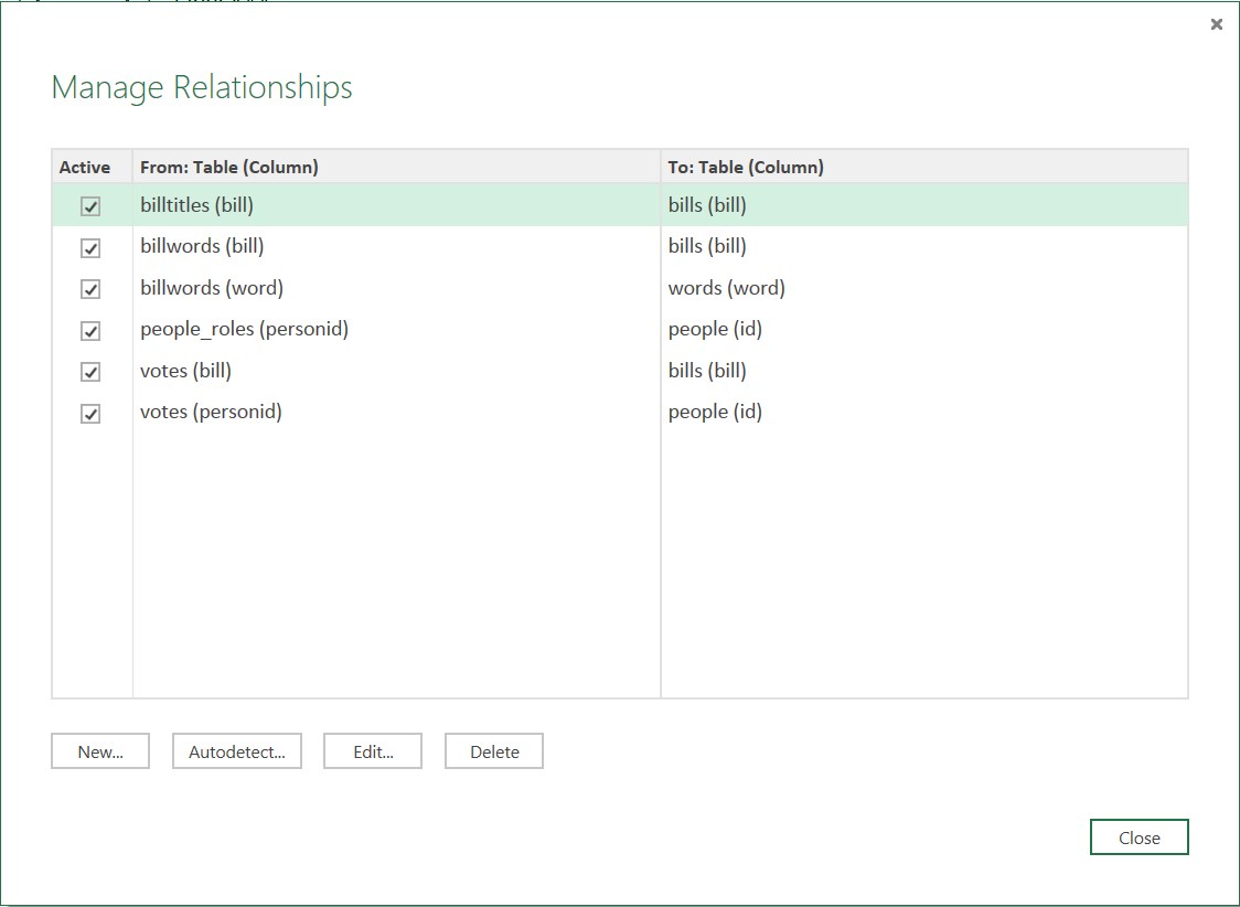
Switch to Report in the bottom-left to load your data into your data model. Make sure that your data model relationships look like the following by clicking on “Manage” in the “Relationships“ section of the ribbon.
Home stretch, add a tree map to your report based upon “word” and “count” in “words” and then whatever slicers and other report elements you desire.