C# Parallel Processing Case Study – Simple One Dimensional Integration

In this very short article we use the both of the parallel processing facilities found in C# .NET Framework 4.5.2, namely multitasking and parallel loops. We use the one dimensional trapezoidal integration technique with or without error correction. This is the simplest all basic numerical integration formulas and due to the slow convergence of the technique we can give our sequential and non-sequential methods time to do some work.

First a word about our computer system. All experiments mentioned in this article were run on a relatively new (late October 2015) Dell XPS 8900 computer with an Intel Core i7-6700K CPU operating at a clock frequency of 4.00 GHz with 16 GB DDR4 memory and a 2 TB hard-drive with a 32 GB SSD buffer. The code was compiled and ran in Debug mode within the Visual Studio 2015 Community version.

The trapezoidal rule is the first of the class of integration formulas known as the closed Newton-Cotes formulas and is given by the following equation:

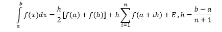
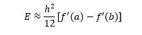
Looking at the formula there are two obvious ways of introducing parallel processing to the integration algorithm: breaking the summation into a number of concurrent summing tasks or a parallel loop over the summation. We implement both of these suggestions in a C# application. If the derivative of integrand is easily calculable then an approximate error correcting term can be added to the preceding formula:

Our integration code base consists of six versions of the trapezoidal integration algorithm:

1. Sequential without error correction

2. Sequential with error correction

3. Parallel loop without error correction

4. Parallel loop with error correction

5. Multitasking without error correction

6. Multitasking with error correction

The code for the sequential versions are given next:

public double  SeqTrapezoidalRule(
   double a, double b, int n,
   Func<double, double> f)
// a and b are the endpoints
// n is the number of steps
// f is f(x)
{
    double h = (b - a) / (n + 1);
    double sum = 0.5 * (f(a) + f(b));
 
    for (int i = 1; i <= n; i++)
    {
        sum += f(a + i * h);
    }
 
    return h * sum;
}
 
public double  SeqTrapezoidalRuleWithCorrection(
    double a, double b, int n,
    Func<double, double> f, Func<double, double> fp)
// a and b are the endpoints
// n is the number of steps
// f is f(x) and fp  is the derivative of f f'(x)
{
    double h = (b - a) / (n + 1);
    double sum = 0.5 * (f(a) + f(b));
 
    for (int i = 1; i <= n; i++)
    {
        sum += f(a + i * h);
    }
 
    return h * (sum + h * (fp(a) - fp(b)) / 12.0);
}

Now we display the parallel loop variants:

public double  ParTrapezoidalRule(
   double a, double b, int n,
   Func<double, double> f)
// a and b are the endpoints
// n is the number of steps
// f is f(x)
{
    double h = (b - a) / (n + 1);
    double sum = 0.5 * (f(a) + f(b));
    double[] innerSum = new  double[n + 1];
 
    Parallel.For(1, n + 1, i =>
    {
        innerSum[i] = f(a + i * h);
    });
 
 
    for (int j = 1; j <= n; j++)
        sum += innerSum[j];
 
    return h * sum;
}
 
public double  ParTrapezoidalRuleWithCorrection(
   double a, double b, int n,
   Func<double, double> f, Func<double, double> fp)
// a and b are the endpoints
// n is the number of steps
// f is f(x) and fp  is the derivative of f f'(x)
{
    double h = (b - a) / (n + 1);
    double sum = 0.5 * (f(a) + f(b));
    double[] innerSum = new  double[n + 1];
 
    Parallel.For(1, n + 1, i =>
    {
        innerSum[i] = f(a + i * h);
    });
 
 
    for (int j = 1; j <= n; j++)
        sum += innerSum[j];
 
    return h * (sum + h * (fp(a) - fp(b)) / 12.0);
}

And finally we show the multitasking methods:

public struct  State
{
    public double  a, h;
    public int  steps;
    public Func<double, double> f;
    public List<double> sum;
 
    public State(double a, double h, int steps, Func<double, double> f)
    {
        this.a = a;
        this.h = h;
        this.steps = steps;
        this.f = f;
        sum = new  List<double>();
    }
}
 
public void  SumTask(object  o)
{
    State s = (State)o;
    double sum = 0;
 
    for (int i = 1; i <= s.steps; i++)
    {
        sum += s.f(s.a + i * s.h);
    }
 
    s.sum.Add(sum);
}
 
public double  TasTrapezoidalRule(
  double a, double b, int cores, int n,
  Func<double, double> f)
// a and b are the endpoints
// cores is the number of physical processors
// n is the number of steps must be a multiple of cores
// f is f(x)
{
    double h = (b - a) / (n + 1);
    double sum = 0.5 * (f(a) + f(b));
    int steps = n / cores;
    State[] states = new  State[cores]; 
    Task[] tasks = new  Task[cores];
 
    for (int i = 0; i < cores; i++)
    {
        states[i] = new  State(a + i * h * steps, h, steps, f);
        tasks[i] = new  Task(SumTask, states[i]);
        tasks[i].Start();
    }
 
    Task.WaitAll(tasks);
 
    for (int i = 0; i < cores; i++)
    {
        sum += states[i].sum[0];
    }
 
    return h * sum;
}
 
public double  TasTrapezoidalRuleWithCorrection(
  double a, double b, int cores, int n,
  Func<double, double> f, Func<double, double> fp)
// a and b are the endpoints
// cores is the number of physical processors
// n is the number of steps must be a multiple of cores
// f is f(x) and fp  is the derivative of f f'(x)
{
    double h = (b - a) / (n + 1);
    double sum = 0.5 * (f(a) + f(b));
    int steps = n / cores;
    State[] states = new  State[cores];
    Task[] tasks = new  Task[cores];
 
    for (int i = 0; i < cores; i++)
    {
        states[i] = new  State(a + i * h * steps, h, steps, f);
        tasks[i] = new  Task(SumTask, states[i]);
        tasks[i].Start();
    }
 
    Task.WaitAll(tasks);
 
    for (int i = 0; i < cores; i++)
    {
        sum += states[i].sum[0];
    }
 
    return h * (sum + h * (fp(a) - fp(b)) / 12.0);
}

The “cores” parameter is four on our computer’s architecture. At this point we must mention the four test definite integrals used in our numerical computations:

The numerical values of the first and second were found using the Wolfram online definite integral calculator. The third integral can be easily calculated using integration by parts. The last integral is well known to every competent student of elementary calculus. We only require 15 decimal point accuracy of our application.

The following tables summarize our results on the four preceding definite integrals:

So it seems that the multitasking version has the best rounding characteristics in most cases although at a runtime cost. It would be interesting to see which method is best for a definite integral computationally intense program.