The Jacobi Relaxation: an Instance of Data Parallelism
In this entry, I will describe an important parallel programming concept, data parallelism. I will then show data parallelism in action by presenting a simplified implementation of the Jacobi Relaxation algorithm.
Data Parallelism
In general, data parallelism occurs in algorithms where the same set of steps is applied to multiple chunks of data independently and simultaneously. This type of algorithm is also sometimes referred to as “embarrassingly parallel”. It implies no data dependencies, meaning that the algorithm can be applied to different chunks of data in any order and still achieve correct results. This differs from task parallelism, where cross-thread communication, ordered data dependencies (e.g. in a workflow), and branching behavior are commonplace.
It is important for anyone writing parallel programs to understand the differences between data and task parallelism and to be able to recognize them when they see them. The type of parallelism involved with your algorithm can have drastic implications on how it can be implemented, both in terms of correctness and performance.
The Simplified Jacobi Relaxation Algorithm
The Jacobi Relaxation is an iterative algorithm that is used to approximate Laplace differential equations. The Jacobi Relaxation technique can be used in a variety of applications, including the simulation of temperature transfer (as we’ll see shortly). For more information about relaxations, and approximating Laplace differentials, see https://www.damtp.cam.ac.uk/lab/people/sd/lectures/nummeth98/pdes.htm.
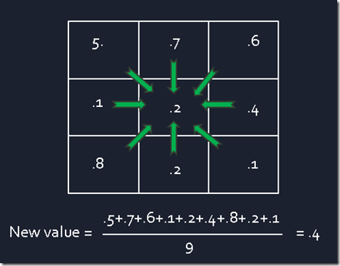
Here I will describe a, simple, two-dimensional implementation. In my implementation I create two, two-dimensional double arrays. I update each element in the array by taking the average of each element with its eight neighbors (see figure 1). I read the values from one array, calculate the average, and then write the calculated average into the corresponding element in the second array. This operation is performed on every element of the array constituting a single iteration. This process is then executed repeatedly over numerous iterations.

Figure 1: Example calculation – the center element’s value is updated based on an average of itself and its eight neighbors
Below is a simplified code snippet illustrating the set of steps described in the paragraph above. Note that “size” is the length and width of the underlying 2-d arrays; “oldgrid” and “grid” are the first and second arrays on which the calculations are performed. The if-statements simply perform bounds-checking to handle the elements around the perimeter of the array.
for (int i = 0; i < iterations; i++)
{
for (int x = 0; x < size; x++)
{
for (int y = 0; y < size; y++)
{
int denom = 1;
double sum = oldGrid[x, y];
//left neighbor
if (x > 0)
{
sum += oldGrid[x - 1, y];
denom++;
}
//right neighbor
if (x < size - 1)
{
sum += oldGrid[x + 1, y];
denom++;
}
//upper neighbor
if (y > 0)
{
sum += oldGrid[x, y - 1];
denom++;
}
//lower neighbor
if (y < size - 1)
{
sum += oldGrid[x, y + 1];
denom++;
}
//left-upper neighbor
if ((x > 0) && (y > 0))
{
sum += oldGrid[x - 1, y - 1];
denom++;
}
//right-upper neighbor
if ((x < size - 1) && (y > 0))
{
sum += oldGrid[x + 1, y - 1];
denom++;
}
//right-lower neighbor
if ((x < size - 1) && (y < size - 1))
{
sum += oldGrid[x + 1, y + 1];
denom++;
}
//left-lower neighbor
if ((x > 0) && (y < size - 1))
{
sum += oldGrid[x - 1, y + 1];
denom++;
}
grid[x, y] = sum / denom;
}
}
grid[size / 2, size / 2] = 1;//maintain the center point's value
//swap the pointers of the first and second array; this will ensure that the next
//iteration will rely on the values calculated in this iteration
double[,] temp = grid;
grid = oldGrid;
oldGrid = temp;
}
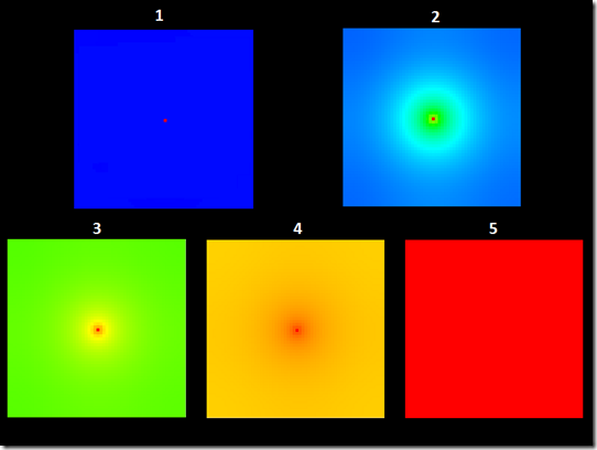
To visually depict this activity I added a heat map. In this case, I define the values in the array to be doubles between 0 and 1. Lower values represent cooler temperatures while higher values represent warmer temperatures. I initialize the input array of the simulation with all but one value set to 0. The element in the center of the input array is set to 1, in order to simulate the spread of heat from a single hot point in a 2-d plane. Throughout the simulation, all values are continually updated except for this specific cell, which remains fixed (at 1). At the beginning of the simulation, you’ll see that image is all blue, except for the single element in the middle which is red. As time progresses, this warm temperature spreads throughout the area causing the image to change color. Figure two illustrates five successive points during the simulation, depicting the change of temperature over time.

Figure 2: Changing values across iterations
So how is this Parallelized?
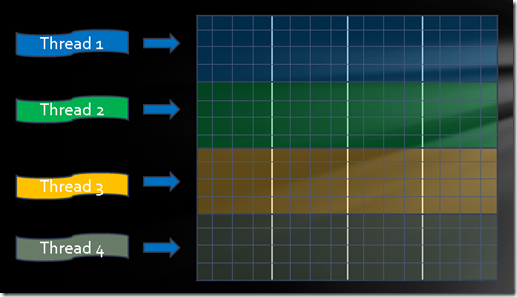
There are many ways to parallelize this algorithm. The simplest way is to create as many threads as there are cores on the machine, where each thread performs this algorithm for a subsection of the array. For example, if your machine has four cores, you could create four threads and let them each operate on one fourth of the rows concurrently (see figure 3). This is known as a row-decomposition. In this way, each thread iterates through one fourth of the overall array and updates the values of the cells in its own set of rows.

Figure 3: A four-way row decomposition for parallel execution on a 16x16 array
What I’ve been discussing so far is how to parallelize the work done within a single iteration, so I’d also like to point out what isn’t parallelizable here: that multiple iterations cannot be calculated concurrently. As an example, the second and fifth iterations cannot be executed concurrently because any single iteration depends on the values calculated in the previous iteration. Therefore, the flow of this program works by performing the work for a fixed iteration in parallel, waiting until all threads have finished their work (aka join), and only then moving forward to the next iteration by re-spawning the appropriate number of threads. It’s important to understand that some aspects of this algorithm are parallelizable while others are not.
What makes this Data Parallel?
This algorithm exhibits data parallelism due to the fact that the same set of steps are applied to multiple pieces of data. In this case, the procedure is an average being computed and the different pieces of data are the various elements of the array.
It is critical to be able to spot data parallelism when you see it because data parallel algorithms allow the developer to more easily construct efficient and safe code. As opposed to the more complex solutions employed against task parallelism, data parallelism allows the programmer to perform the same operation on each piece of data concurrently without concern for race conditions and consequently, the need for synchronization, which results in significant performance overhead. Arguably, data parallel algorithms perform better (due to the lack of synchronization) and are easier for the developer to implement.
Conclusion
For this algorithm, it is important to understand which aspects of it are parallelizable and which aspects of the algorithm are not parallelizable. It’s also important to understand the type of parallelism involved. As I mentioned, the act of computing averages within a fixed iteration is parallelizable, however, it is not possible to compute multiple iterations in parallel. In addition, the algorithm used to parallelize the computation is data parallel. I hope you can take this example and apply it to a variety of problems to understand what can and cannot be parallelized, as well as what type of parallelism is involved.
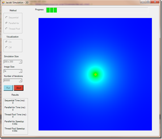
For a more in-depth look at my implementation of this algorithm, you can download the demo from our Code Gallery page; to download it directly, click here. This demo allows you to visualize the results of the Jacobi Relaxation with three different implementations: sequentially, in parallel using the .NET thread pool, and in parallel using the Task Parallel Library’s (TPL) parallel for-loop (see figure 4). It’s interesting to compare the timing of the trials by adjusting the simulation size (the size of the underlying 2-d array) and the number of iterations. You’ll find that the speedups improve as the size of the simulation increases. This results from a decreased communication to computation ratio as the underlying matrix grows. It’s also worth looking at the difference in the sequential and TPL implementations (I’ll give you a hint: there’s very little difference at all!).

Figure 4: A demo of my Jacobi Relaxation implementation
Enjoy!
James Rapp – Parallel Computing Platform