Analyzing Stock Price Data with Sho, Part I
One fun arena for doing data analysis and visualization is the stock market. Fortunately, a lot of stock market data is now available publicly, and Sho makes it easy and fun to do various kinds of analysis on it. We’ll look at data from the stocks in the S&P 500 index, since that data is readily available – you can get the last year of daily prices from various locations, including https://pages.swcp.com/stocks/#Daily%20update.
Start by downloading the data – pick the “Historical” option and click “Get Full Set;” this will give you a zip file which will contain a single file, sp500hst.txt. Save that to some handy directory. If we open up that file in a text editor, we’ll see a bunch of lines like the below:
20100310,CBS,14.45,14.75,14.39,14.75,81612
20100311,CBS,14.63,14.8,14.4,14.8,65851
20100312,CBS,14.79,14.85,14.42,14.6,66466
20100315,CBS,14.52,14.535,14.22,14.44,68313
20100316,CBS,14.44,14.78,14.31,14.78,103030
20100317,CBS,14.83,14.945,14.46,14.5,80747
20100318,CBS,14.51,14.655,14.24,14.37,55267
20100319,CBS,14.42,14.63,13.98,13.98,99261
20100322,CBS,13.96,14.14,13.7,14.07,58456
20100323,CBS,14.14,14.28,14.06,14.26,66844
20100324,CBS,14.13,14.43,14.03,14.24,84188
20100325,CBS,14.42,14.44,13.85,13.87,108878
In other words, the date, followed by the symbol, followed by open, high, low, close, and the volume for that day. We’re interested in grabbing the closing value for each day for a given stock so that we can plot it, compute running averages, make predictions, etc. Let’s write a function that will extract this from the file:
def getseries(symbol, filename):
data = csvreadArray(filename)
dates = []
prices = []
for line in data.Rows:
if line[1] == symbol:
dates.Add(line[0]) # date
prices.Add(float(line[5])) # closing price
return(dates,DoubleArray.From(prices))
This will get us the dates and closing price for a given symbol. Note that we convert the list of prices to a DoubleArray for ease of later manipulations. Let’s retrieve the prices for symbol “CBS” and plot the result:
>>> dates, prices = getseries("CBS", "c:/mypath/sp500hst.txt")
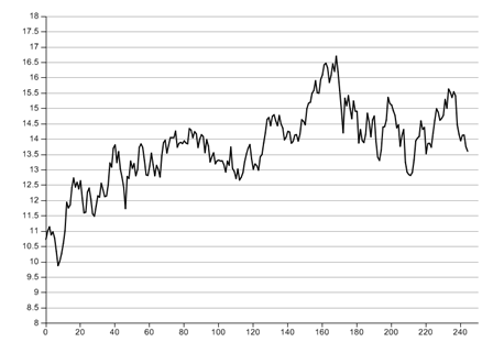
>>> plot(prices)
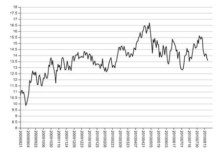
That gives us a first look at the raw data. Note that the x axis labels are just the index number of each element; we’d rather see the appropriate date labels for the x axis, but since they’re strings and not numeric values, we can’t just pass them in via plot(x,y). We can instead modify the x-axis labels with the xlabels command – we just need to tell it which locations to label and what the respective values would be, so we’ll create a series of numbers spaced by 10 and then pick out the appropriate labels with a list comprehension:
>>> sd = range(0,len(dates),10)
>>> xlabels(sd, [dates[ind] for ind in sd], orientation=90) # create date labels on x axis and turn them 90 degrees
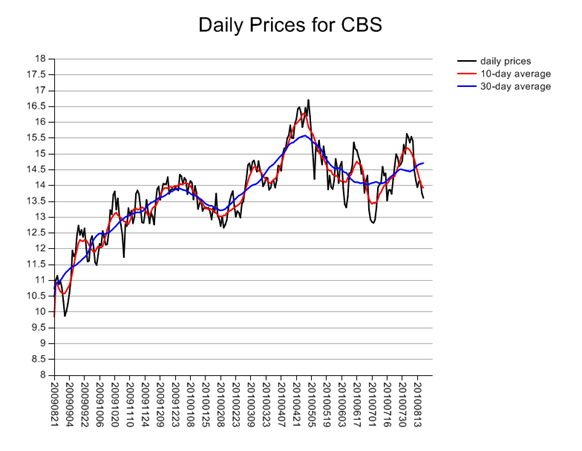
Now we’d like to see the moving averages over different windows for the stock in addition to its daily value. We can use the signal processing tools in Sho to easily compute a moving average by convolving the time series with a box filter, which we can represent via ones(N,1)/N where N is the length of the filter. We divide by N to normalize the sum of the filter to 1. We’ll compute a 10-day and a 30-day moving average.
>>> smooth10 = SignalProc.conv(DoubleArray.From(prices).T, ones(10,1)/10.0, CompMode.Auto, BoundaryMode.Reflect)
>>> smooth30 = SignalProc.conv(DoubleArray.From(prices).T, ones(30,1)/30.0, CompMode.Auto, BoundaryMode.Reflect)
We’ll now plot these smoothed signals on top of the original prices by using the hold() command to hold the previous plot. Finally, we’ll add a legend to label the separate time series; we’ll also add a title for good measure.
>>> hold()
>>> plot(smooth10)
>>> plot(smooth30)
>>> legend('daily prices','10-day average','30-day average')
>>> plottitle('Daily Prices for CBS')
That gets us to the plot below:
In the next post, we’ll show how build a simple autoregressive model for predicting future prices (though not with particularly high accuracy).
Comments
Anonymous
August 29, 2011
Keep up the great work on your blog. http://chasingbeta.com/Anonymous
February 15, 2012
The comment has been removedAnonymous
October 31, 2013
Are you using Microsoft Excel, Access to write these formulas??? Tom


