리소스 추정기를 실행하는 다양한 방법
이 문서에서는 Azure Quantum 리소스 추정기를 사용하는 방법을 알아봅니다. 리소스 추정기는 Quantum 개발 키트의 일부이며 다양한 플랫폼 및 IDE에서 사용할 수 있습니다.
Q# 프로그램을 실행하는 경우 Resource Estimator는 Quantum Development Kit 확장을 사용하여 Visual Studio Code에서 사용할 수 있습니다. Visual Studio Code에서 리소스 추정기를 사용하기 위해 Azure 구독이 있어야 하는 것은 아닙니다.
Qiskit 또는 QIR 프로그램을 실행하는 경우 Azure Portal에서 리소스 추정기를 사용할 수 있으며 이를 사용하려면 Azure 구독이 필요합니다.
다음 표에서는 리소스 추정기를 실행하는 다양한 방법을 보여줍니다.
| 사용자 시나리오 | 플랫폼 | 자습서 |
|---|---|---|
| Q# 프로그램의 리소스 예측 | Visual Studio Code | 페이지 맨 위에 있는 VS Code에서 Q#을 선택합니다. |
| Q# 프로그램의 리소스 예측(고급) | Visual Studio Code의 Jupyter Notebook | 페이지 맨 위에 있는 Jupyter Notebook에서 Q#을 선택합니다. |
| Qiskit 프로그램의 리소스 예측 | Azure Portal | 페이지 맨 위에 있는 Azure Portal에서 Qiskit 선택 |
| QIR 프로그램의 리소스 예측 | Azure Portal | QIR 제출 |
| FCIDUMP 파일을 인수 매개 변수로 사용(고급) | Visual Studio Code | 양자 화학 문제 제출 |
VS Code의 필수 구성 요소
- 최신 버전의 Visual Studio Code 또는 웹에서 VS Code를 엽니다.
- 최신 버전의 Azure Quantum 개발 키트 확장. 설치 세부 정보는 VS Code에 QDK 설치를 참조 하세요.
팁
로컬 리소스 추정기를 실행하기 위해 Azure 계정이 필요하지 않습니다.
새 Q# 파일 만들기
- Visual Studio Code를 열고 파일>새 텍스트 파일을 선택하여 새 파일을 만듭니다.
- 파일을
ShorRE.qs로 저장합니다. 이 파일에는 프로그램에 대한 Q# 코드가 포함됩니다.
양자 알고리즘 생성
다음 코드를 파일에 복사합니다 ShorRE.qs .
namespace Shors {
    open Microsoft.Quantum.Arrays;
    open Microsoft.Quantum.Canon;
    open Microsoft.Quantum.Convert;
    open Microsoft.Quantum.Diagnostics;
    open Microsoft.Quantum.Intrinsic;
    open Microsoft.Quantum.Math;
    open Microsoft.Quantum.Measurement;
    open Microsoft.Quantum.Unstable.Arithmetic;
    open Microsoft.Quantum.ResourceEstimation;

    @EntryPoint()
    operation RunProgram() : Unit {
        let bitsize = 31;

        // When choosing parameters for `EstimateFrequency`, make sure that
        // generator and modules are not co-prime
        let _ = EstimateFrequency(11, 2^bitsize - 1, bitsize);
    }

    // In this sample we concentrate on costing the `EstimateFrequency`
    // operation, which is the core quantum operation in Shors algorithm, and
    // we omit the classical pre- and post-processing.

    /// # Summary
    /// Estimates the frequency of a generator
    /// in the residue ring Z mod `modulus`.
    ///
    /// # Input
    /// ## generator
    /// The unsigned integer multiplicative order (period)
    /// of which is being estimated. Must be co-prime to `modulus`.
    /// ## modulus
    /// The modulus which defines the residue ring Z mod `modulus`
    /// in which the multiplicative order of `generator` is being estimated.
    /// ## bitsize
    /// Number of bits needed to represent the modulus.
    ///
    /// # Output
    /// The numerator k of dyadic fraction k/2^bitsPrecision
    /// approximating s/r.
    operation EstimateFrequency(
        generator : Int,
        modulus : Int,
        bitsize : Int
    )
    : Int {
        mutable frequencyEstimate = 0;
        let bitsPrecision =  2 * bitsize + 1;

        // Allocate qubits for the superposition of eigenstates of
        // the oracle that is used in period finding.
        use eigenstateRegister = Qubit[bitsize];

        // Initialize eigenstateRegister to 1, which is a superposition of
        // the eigenstates we are estimating the phases of.
        // We first interpret the register as encoding an unsigned integer
        // in little endian encoding.
        ApplyXorInPlace(1, eigenstateRegister);
        let oracle = ApplyOrderFindingOracle(generator, modulus, _, _);

        // Use phase estimation with a semiclassical Fourier transform to
        // estimate the frequency.
        use c = Qubit();
        for idx in bitsPrecision - 1..-1..0 {
            within {
                H(c);
            } apply {
                // `BeginEstimateCaching` and `EndEstimateCaching` are the operations
                // exposed by Azure Quantum Resource Estimator. These will instruct
                // resource counting such that the if-block will be executed
                // only once, its resources will be cached, and appended in
                // every other iteration.
                if BeginEstimateCaching("ControlledOracle", SingleVariant()) {
                    Controlled oracle([c], (1 <<< idx, eigenstateRegister));
                    EndEstimateCaching();
                }
                R1Frac(frequencyEstimate, bitsPrecision - 1 - idx, c);
            }
            if MResetZ(c) == One {
                set frequencyEstimate += 1 <<< (bitsPrecision - 1 - idx);
            }
        }

        // Return all the qubits used for oracles eigenstate back to 0 state
        // using Microsoft.Quantum.Intrinsic.ResetAll.
        ResetAll(eigenstateRegister);

        return frequencyEstimate;
    }

    /// # Summary
    /// Interprets `target` as encoding unsigned little-endian integer k
    /// and performs transformation |k⟩ ↦ |gᵖ⋅k mod N ⟩ where
    /// p is `power`, g is `generator` and N is `modulus`.
    ///
    /// # Input
    /// ## generator
    /// The unsigned integer multiplicative order ( period )
    /// of which is being estimated. Must be co-prime to `modulus`.
    /// ## modulus
    /// The modulus which defines the residue ring Z mod `modulus`
    /// in which the multiplicative order of `generator` is being estimated.
    /// ## power
    /// Power of `generator` by which `target` is multiplied.
    /// ## target
    /// Register interpreted as little endian encoded which is multiplied by
    /// given power of the generator. The multiplication is performed modulo
    /// `modulus`.
    internal operation ApplyOrderFindingOracle(
        generator : Int, modulus : Int, power : Int, target : Qubit[]
    )
    : Unit
    is Adj + Ctl {
        // The oracle we use for order finding implements |x⟩ ↦ |x⋅a mod N⟩. We
        // also use `ExpModI` to compute a by which x must be multiplied. Also
        // note that we interpret target as unsigned integer in little-endian
        // encoding.
        ModularMultiplyByConstant(modulus,
                                    ExpModI(generator, power, modulus),
                                    target);
    }

    /// # Summary
    /// Performs modular in-place multiplication by a classical constant.
    ///
    /// # Description
    /// Given the classical constants `c` and `modulus`, and an input
    /// quantum register  |𝑦⟩, this operation
    /// computes `(c*x) % modulus` into |𝑦⟩.
    ///
    /// # Input
    /// ## modulus
    /// Modulus to use for modular multiplication
    /// ## c
    /// Constant by which to multiply |𝑦⟩
    /// ## y
    /// Quantum register of target
    internal operation ModularMultiplyByConstant(modulus : Int, c : Int, y : Qubit[])
    : Unit is Adj + Ctl {
        use qs = Qubit[Length(y)];
        for (idx, yq) in Enumerated(y) {
            let shiftedC = (c <<< idx) % modulus;
            Controlled ModularAddConstant([yq], (modulus, shiftedC, qs));
        }
        ApplyToEachCA(SWAP, Zipped(y, qs));
        let invC = InverseModI(c, modulus);
        for (idx, yq) in Enumerated(y) {
            let shiftedC = (invC <<< idx) % modulus;
            Controlled ModularAddConstant([yq], (modulus, modulus - shiftedC, qs));
        }
    }

    /// # Summary
    /// Performs modular in-place addition of a classical constant into a
    /// quantum register.
    ///
    /// # Description
    /// Given the classical constants `c` and `modulus`, and an input
    /// quantum register  |𝑦⟩, this operation
    /// computes `(x+c) % modulus` into |𝑦⟩.
    ///
    /// # Input
    /// ## modulus
    /// Modulus to use for modular addition
    /// ## c
    /// Constant to add to |𝑦⟩
    /// ## y
    /// Quantum register of target
    internal operation ModularAddConstant(modulus : Int, c : Int, y : Qubit[])
    : Unit is Adj + Ctl {
        body (...) {
            Controlled ModularAddConstant([], (modulus, c, y));
        }
        controlled (ctrls, ...) {
            // We apply a custom strategy to control this operation instead of
            // letting the compiler create the controlled variant for us in which
            // the `Controlled` functor would be distributed over each operation
            // in the body.
            //
            // Here we can use some scratch memory to save ensure that at most one
            // control qubit is used for costly operations such as `AddConstant`
            // and `CompareGreaterThenOrEqualConstant`.
            if Length(ctrls) >= 2 {
                use control = Qubit();
                within {
                    Controlled X(ctrls, control);
                } apply {
                    Controlled ModularAddConstant([control], (modulus, c, y));
                }
            } else {
                use carry = Qubit();
                Controlled AddConstant(ctrls, (c, y + [carry]));
                Controlled Adjoint AddConstant(ctrls, (modulus, y + [carry]));
                Controlled AddConstant([carry], (modulus, y));
                Controlled CompareGreaterThanOrEqualConstant(ctrls, (c, y, carry));
            }
        }
    }

    /// # Summary
    /// Performs in-place addition of a constant into a quantum register.
    ///
    /// # Description
    /// Given a non-empty quantum register |𝑦⟩ of length 𝑛+1 and a positive
    /// constant 𝑐 < 2ⁿ, computes |𝑦 + c⟩ into |𝑦⟩.
    ///
    /// # Input
    /// ## c
    /// Constant number to add to |𝑦⟩.
    /// ## y
    /// Quantum register of second summand and target; must not be empty.
    internal operation AddConstant(c : Int, y : Qubit[]) : Unit is Adj + Ctl {
        // We are using this version instead of the library version that is based
        // on Fourier angles to show an advantage of sparse simulation in this sample.

        let n = Length(y);
        Fact(n > 0, "Bit width must be at least 1");

        Fact(c >= 0, "constant must not be negative");
        Fact(c < 2 ^ n, $"constant must be smaller than {2L ^ n}");

        if c != 0 {
            // If c has j trailing zeroes than the j least significant bits
            // of y won't be affected by the addition and can therefore be
            // ignored by applying the addition only to the other qubits and
            // shifting c accordingly.
            let j = NTrailingZeroes(c);
            use x = Qubit[n - j];
            within {
                ApplyXorInPlace(c >>> j, x);
            } apply {
                IncByLE(x, y[j...]);
            }
        }
    }

    /// # Summary
    /// Performs greater-than-or-equals comparison to a constant.
    ///
    /// # Description
    /// Toggles output qubit `target` if and only if input register `x`
    /// is greater than or equal to `c`.
    ///
    /// # Input
    /// ## c
    /// Constant value for comparison.
    /// ## x
    /// Quantum register to compare against.
    /// ## target
    /// Target qubit for comparison result.
    ///
    /// # Reference
    /// This construction is described in [Lemma 3, arXiv:2201.10200]
    internal operation CompareGreaterThanOrEqualConstant(c : Int, x : Qubit[], target : Qubit)
    : Unit is Adj+Ctl {
        let bitWidth = Length(x);

        if c == 0 {
            X(target);
        } elif c >= 2 ^ bitWidth {
            // do nothing
        } elif c == 2 ^ (bitWidth - 1) {
            ApplyLowTCNOT(Tail(x), target);
        } else {
            // normalize constant
            let l = NTrailingZeroes(c);

            let cNormalized = c >>> l;
            let xNormalized = x[l...];
            let bitWidthNormalized = Length(xNormalized);
            let gates = Rest(IntAsBoolArray(cNormalized, bitWidthNormalized));

            use qs = Qubit[bitWidthNormalized - 1];
            let cs1 = [Head(xNormalized)] + Most(qs);
            let cs2 = Rest(xNormalized);

            within {
                for i in IndexRange(gates) {
                    (gates[i] ? ApplyAnd | ApplyOr)(cs1[i], cs2[i], qs[i]);
                }
            } apply {
                ApplyLowTCNOT(Tail(qs), target);
            }
        }
    }

    /// # Summary
    /// Internal operation used in the implementation of GreaterThanOrEqualConstant.
    internal operation ApplyOr(control1 : Qubit, control2 : Qubit, target : Qubit) : Unit is Adj {
        within {
            ApplyToEachA(X, [control1, control2]);
        } apply {
            ApplyAnd(control1, control2, target);
            X(target);
        }
    }

    internal operation ApplyAnd(control1 : Qubit, control2 : Qubit, target : Qubit)
    : Unit is Adj {
        body (...) {
            CCNOT(control1, control2, target);
        }
        adjoint (...) {
            H(target);
            if (M(target) == One) {
                X(target);
                CZ(control1, control2);
            }
        }
    }


    /// # Summary
    /// Returns the number of trailing zeroes of a number
    ///
    /// ## Example
    /// ```qsharp
    /// let zeroes = NTrailingZeroes(21); // = NTrailingZeroes(0b1101) = 0
    /// let zeroes = NTrailingZeroes(20); // = NTrailingZeroes(0b1100) = 2
    /// ```
    internal function NTrailingZeroes(number : Int) : Int {
        mutable nZeroes = 0;
        mutable copy = number;
        while (copy % 2 == 0) {
            set nZeroes += 1;
            set copy /= 2;
        }
        return nZeroes;
    }

    /// # Summary
    /// An implementation for `CNOT` that when controlled using a single control uses
    /// a helper qubit and uses `ApplyAnd` to reduce the T-count to 4 instead of 7.
    internal operation ApplyLowTCNOT(a : Qubit, b : Qubit) : Unit is Adj+Ctl {
        body (...) {
            CNOT(a, b);
        }

        adjoint self;

        controlled (ctls, ...) {
            // In this application this operation is used in a way that
            // it is controlled by at most one qubit.
            Fact(Length(ctls) <= 1, "At most one control line allowed");

            if IsEmpty(ctls) {
                CNOT(a, b);
            } else {
                use q = Qubit();
                within {
                    ApplyAnd(Head(ctls), a, q);
                } apply {
                    CNOT(q, b);
                }
            }
        }

        controlled adjoint self;
    }
}
리소스 예측 도구 실행
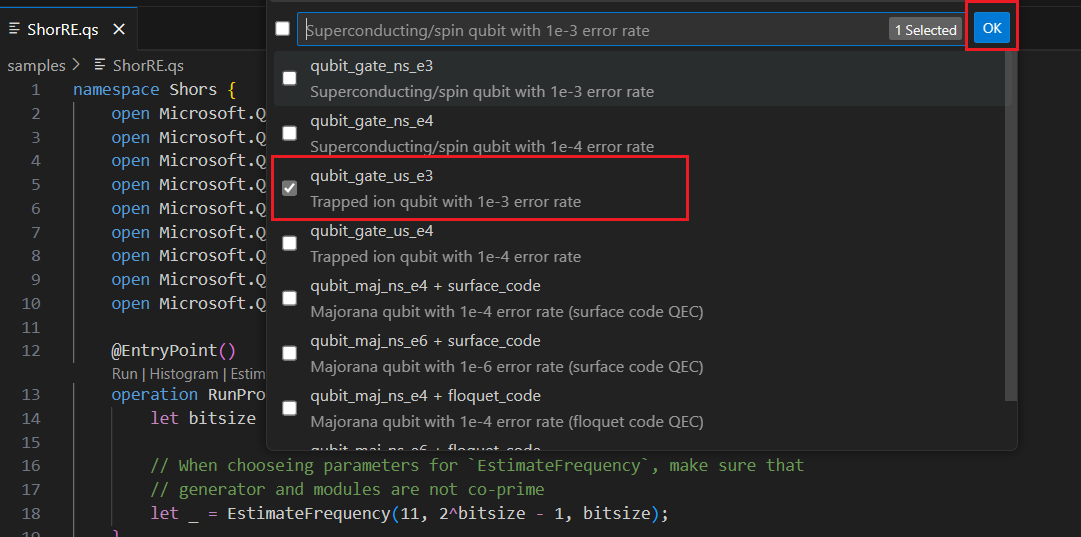
Resource Estimator는 6개의 미리 정의된 큐비트 매개 변수를 제공하며, 그 중 4개에는 게이트 기반 명령 집합이 있고 2개에는 Majorana 명령 집합이 있습니다. 또한 두 개의 양자 오류 수정 코드와 surface_codefloquet_code.
이 예제에서는 큐비트 매개 변수 및 surface_code 양자 오류 수정 코드를 사용하여 qubit_gate_us_e3 리소스 추정기를 실행합니다.
보기 - 명령 팔레트를 선택하고 Q#: 자원 예측 계산 옵션을 표시해야 하는 "리소스"를 입력합니다.> 아래
@EntryPoint()명령 목록에서 견적을 클릭할 수도 있습니다. 자원 추정기 창을 열려면 이 옵션을 선택합니다.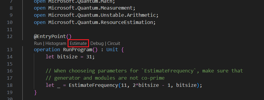
하나 이상의 Qubit 매개 변수 + 오류 수정 코드 형식을 선택하여 리소스를 예측할 수 있습니다. 이 예제에서는 qubit_gate_us_e3 선택하고 확인을 클릭합니다.
오류 예산을 지정하거나 기본값 0.001을 적용합니다. 이 예제에서는 기본값을 그대로 두고 Enter 키를 누릅니 다.
Enter 키를 눌러 파일 이름(이 경우 ShorRE)에 따라 기본 결과 이름을 적용합니다.
결과 보기
리소스 추정기는 동일한 알고리즘에 대한 여러 예상치를 제공하며, 각 알고리즘은 큐비트 수와 런타임 간의 절충을 보여 줍니다. 런타임과 시스템 규모 간의 장단점 이해는 리소스 예측의 더 중요한 측면 중 하나입니다.
리소스 예측 결과는 Q# 추정 창에 표시됩니다.
결과 탭에는 리소스 예측에 대한 요약이 표시됩니다. 첫 번째 행 옆의 아이콘 을 클릭하여 표시할 열을 선택합니다. 실행 이름, 예측 형식, 큐비트 유형, qec 체계, 오류 예산, 논리 큐비트, 논리 깊이, 코드 거리, T 상태, T 팩터리, T 팩터리 분수, 런타임, rQOPS 및 실제 큐비트 중에서 선택할 수 있습니다.
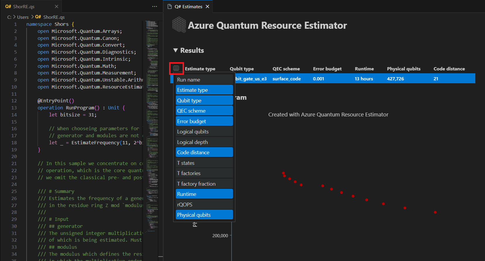
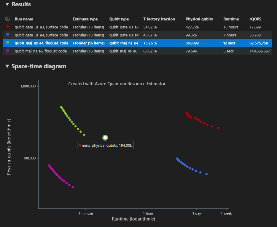
결과 테이블의 추정 형식 열에서 알고리즘에 대한 {큐비트 수, 런타임}의 최적 조합 수를 확인할 수 있습니다. 이러한 조합은 시공간 다이어그램에서 볼 수 있습니다.
시공간 다이어그램은 실제 큐비트 수와 알고리즘의 런타임 간의 장단점이 표시됩니다. 이 경우 리소스 추정기는 수천 가지 가능한 조합 중 13가지 최적의 조합을 찾습니다. 각 {큐비트 수, 런타임} 지점을 마우스로 가리키면 해당 시점에서 리소스 예측의 세부 정보를 볼 수 있습니다.
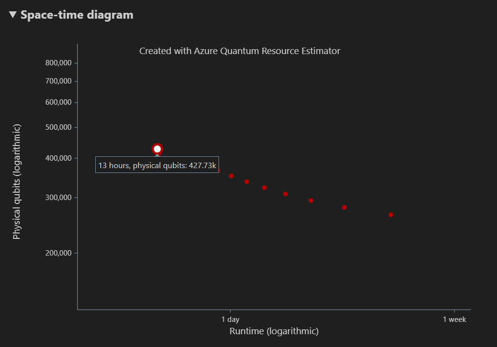
자세한 내용은 시공간 다이어그램을 참조 하세요.
참고 항목
공간 다이어그램과 해당 지점에 해당하는 리소스 예측의 세부 정보를 보려면 {큐비트 수, 런타임} 쌍인 시공간 다이어그램의 한 지점을 클릭해야 합니다.
공간 다이어그램은 알고리즘에 사용되는 실제 큐비트와 {수의 큐비트, 런타임} 쌍에 해당하는 T 팩터리 분포를 보여 줍니다. 예를 들어 시공간 다이어그램에서 가장 왼쪽 지점을 선택하는 경우 알고리즘을 실행하는 데 필요한 실제 큐비트 수는 427726 196686 알고리즘 큐비트이고 그 중 231040은 T 팩터리 큐비트입니다.
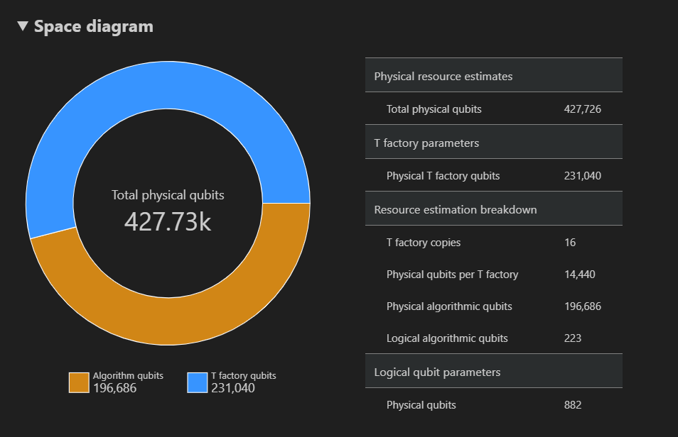
마지막으로 자원 예측 탭에는 {수의 큐비트, 런타임} 쌍에 해당하는 자원 예측 도구에 대한 출력 데이터의 전체 목록이 표시됩니다. 더 많은 정보가 있는 그룹을 축소해 비용 세부 정보를 검사할 수 있습니다. 예를 들어 시공간 다이어그램에서 맨 왼쪽 지점을 선택하고 논리 큐비트 매개 변수 그룹을 축소합니다.
논리적 큐비트 매개 변수 값 QEC 체계 surface_code 코드 거리 21 물리적 큐비트 882 논리적 주기 시간 13밀리초 논리적 큐비트 오류율 3.00E-13 교차 전인자 0.03 오류 수정 임계값 0.01 논리적 주기 시간 수식 (4 * twoQubitGateTime+ 2 *oneQubitMeasurementTime) *codeDistance물리적 큐비트 수식 2 * codeDistance*codeDistance팁
보고서 데이터의 각 출력에 대한 설명을 표시하려면 자세한 행 표시를 클릭합니다.
자세한 내용은 리소스 추정기의 전체 보고서 데이터를 참조 하세요.
target 매개 변수 변경
다른 큐비트 유형, 오류 수정 코드 및 오류 예산을 사용하여 동일한 Q# 프로그램의 비용을 예측할 수 있습니다. 보기 -> 명령 팔레트를 선택하여 리소스 추정기 창을 열고 입력Q#: Calculate Resource Estimates합니다.
Majorana 기반 큐비트 매개 변수 qubit_maj_ns_e6와 같은 다른 구성을 선택합니다. 기본 오류 예산 값을 적용하거나 새 예산 값을 입력하고 Enter 키를 누릅니 다. 리소스 추정기는 새 target 매개 변수를 사용하여 추정을 다시 실행합니다.
자세한 내용은 리소스 예측 도구에 대한 대상 매개 변수를 참조하세요.
매개 변수의 여러 구성 실행
Azure Quantum Resource Estimator는 여러 매개 변수 구성을 target 실행하고 리소스 예측 결과를 비교할 수 있습니다.
보기 - 명령 팔레트를 선택하거나 Ctrl+Shift+P를 누른 다음 입력
Q#: Calculate Resource Estimates합니다.>qubit_gate_us_e3, qubit_gate_us_e4, qubit_maj_ns_e4 + floquet_code 선택하고 qubit_maj_ns_e6 + floquet_code 선택하고 확인을 클릭합니다.
기본 오류 예산 값 0.001을 적용하고 Enter 키를 누릅니 다.
Enter 키를 눌러 입력 파일(이 경우 ShorRE.qs)을 수락합니다.
여러 매개 변수 구성의 경우 결과는 결과 탭의 다른 행에 표시됩니다.
시공간 다이어그램은 매개 변수의 모든 구성에 대한 결과를 보여 줍니다. 결과 테이블의 첫 번째 열에는 매개 변수의 각 구성에 대한 범례가 표시됩니다. 각 지점을 마우스로 가리키면 해당 시점에서 리소스 예측의 세부 정보를 볼 수 있습니다.
시공간 다이어그램의 {수의 큐비트, 런타임} 지점을 클릭하여 해당 공간 다이어그램을 표시하고 데이터를 보고합니다.
VS Code의 Jupyter Notebook에 대한 필수 구성 요소
Python 및 Pip가 설치된 Python 환경입니다.
최신 버전의 Visual Studio Code 또는 웹에서 VS Code를 엽니다.
Azure Quantum Development Kit, Python 및 Jupyter 확장이 설치된 VS Code
최신 Azure Quantum
qsharp및qsharp-widgets패키지입니다.python -m pip install --upgrade qsharp qsharp-widgets
팁
로컬 리소스 추정기를 실행하기 위해 Azure 계정이 필요하지 않습니다.
양자 알고리즘 생성
VS Code에서 명령 팔레트 보기를 > 선택하고 만들기: 새 Jupyter Notebook을 선택합니다.
오른쪽 위에서 VS Code는 Notebook에 대해 선택된 Python 및 가상 Python 환경의 버전을 검색하고 표시합니다. 여러 Python 환경이 있는 경우 오른쪽 위에 있는 커널 선택기를 사용하여 커널을 선택해야 할 수 있습니다. 환경이 검색되지 않은 경우 VS Code의 Jupyter Notebook에서 설정 정보를 참조하세요.
Notebook의 첫 번째 셀에서 패키지를 가져옵니다
qsharp.import qsharp새 셀을 추가하고 다음 코드를 복사합니다.
%%qsharp
open Microsoft.Quantum.Arrays;
open Microsoft.Quantum.Canon;
open Microsoft.Quantum.Convert;
open Microsoft.Quantum.Diagnostics;
open Microsoft.Quantum.Intrinsic;
open Microsoft.Quantum.Math;
open Microsoft.Quantum.Measurement;
open Microsoft.Quantum.Unstable.Arithmetic;
open Microsoft.Quantum.ResourceEstimation;

operation RunProgram() : Unit {
    let bitsize = 31;

    // When choosing parameters for `EstimateFrequency`, make sure that
    // generator and modules are not co-prime
    let _ = EstimateFrequency(11, 2^bitsize - 1, bitsize);
}


// In this sample we concentrate on costing the `EstimateFrequency`
// operation, which is the core quantum operation in Shors algorithm, and
// we omit the classical pre- and post-processing.

/// # Summary
/// Estimates the frequency of a generator
/// in the residue ring Z mod `modulus`.
///
/// # Input
/// ## generator
/// The unsigned integer multiplicative order (period)
/// of which is being estimated. Must be co-prime to `modulus`.
/// ## modulus
/// The modulus which defines the residue ring Z mod `modulus`
/// in which the multiplicative order of `generator` is being estimated.
/// ## bitsize
/// Number of bits needed to represent the modulus.
///
/// # Output
/// The numerator k of dyadic fraction k/2^bitsPrecision
/// approximating s/r.
operation EstimateFrequency(
    generator : Int,
    modulus : Int,
    bitsize : Int
)
: Int {
    mutable frequencyEstimate = 0;
    let bitsPrecision =  2 * bitsize + 1;

    // Allocate qubits for the superposition of eigenstates of
    // the oracle that is used in period finding.
    use eigenstateRegister = Qubit[bitsize];

    // Initialize eigenstateRegister to 1, which is a superposition of
    // the eigenstates we are estimating the phases of.
    // We first interpret the register as encoding an unsigned integer
    // in little endian encoding.
    ApplyXorInPlace(1, eigenstateRegister);
    let oracle = ApplyOrderFindingOracle(generator, modulus, _, _);

    // Use phase estimation with a semiclassical Fourier transform to
    // estimate the frequency.
    use c = Qubit();
    for idx in bitsPrecision - 1..-1..0 {
        within {
            H(c);
        } apply {
            // `BeginEstimateCaching` and `EndEstimateCaching` are the operations
            // exposed by Azure Quantum Resource Estimator. These will instruct
            // resource counting such that the if-block will be executed
            // only once, its resources will be cached, and appended in
            // every other iteration.
            if BeginEstimateCaching("ControlledOracle", SingleVariant()) {
                Controlled oracle([c], (1 <<< idx, eigenstateRegister));
                EndEstimateCaching();
            }
            R1Frac(frequencyEstimate, bitsPrecision - 1 - idx, c);
        }
        if MResetZ(c) == One {
            set frequencyEstimate += 1 <<< (bitsPrecision - 1 - idx);
        }
    }

    // Return all the qubits used for oracle eigenstate back to 0 state
    // using Microsoft.Quantum.Intrinsic.ResetAll.
    ResetAll(eigenstateRegister);

    return frequencyEstimate;
}

/// # Summary
/// Interprets `target` as encoding unsigned little-endian integer k
/// and performs transformation |k⟩ ↦ |gᵖ⋅k mod N ⟩ where
/// p is `power`, g is `generator` and N is `modulus`.
///
/// # Input
/// ## generator
/// The unsigned integer multiplicative order ( period )
/// of which is being estimated. Must be co-prime to `modulus`.
/// ## modulus
/// The modulus which defines the residue ring Z mod `modulus`
/// in which the multiplicative order of `generator` is being estimated.
/// ## power
/// Power of `generator` by which `target` is multiplied.
/// ## target
/// Register interpreted as little endian encoded which is multiplied by
/// given power of the generator. The multiplication is performed modulo
/// `modulus`.
internal operation ApplyOrderFindingOracle(
    generator : Int, modulus : Int, power : Int, target : Qubit[]
)
: Unit
is Adj + Ctl {
    // The oracle we use for order finding implements |x⟩ ↦ |x⋅a mod N⟩. We
    // also use `ExpModI` to compute a by which x must be multiplied. Also
    // note that we interpret target as unsigned integer in little-endian
    // encoding.
    ModularMultiplyByConstant(modulus,
                                ExpModI(generator, power, modulus),
                                target);
}

/// # Summary
/// Performs modular in-place multiplication by a classical constant.
///
/// # Description
/// Given the classical constants `c` and `modulus`, and an input
/// quantum register |𝑦⟩, this operation
/// computes `(c*x) % modulus` into |𝑦⟩.
///
/// # Input
/// ## modulus
/// Modulus to use for modular multiplication
/// ## c
/// Constant by which to multiply |𝑦⟩
/// ## y
/// Quantum register of target
internal operation ModularMultiplyByConstant(modulus : Int, c : Int, y : Qubit[])
: Unit is Adj + Ctl {
    use qs = Qubit[Length(y)];
    for (idx, yq) in Enumerated(y) {
        let shiftedC = (c <<< idx) % modulus;
        Controlled ModularAddConstant([yq], (modulus, shiftedC, qs));
    }
    ApplyToEachCA(SWAP, Zipped(y, qs));
    let invC = InverseModI(c, modulus);
    for (idx, yq) in Enumerated(y) {
        let shiftedC = (invC <<< idx) % modulus;
        Controlled ModularAddConstant([yq], (modulus, modulus - shiftedC, qs));
    }
}

/// # Summary
/// Performs modular in-place addition of a classical constant into a
/// quantum register.
///
/// # Description
/// Given the classical constants `c` and `modulus`, and an input
/// quantum register  |𝑦⟩, this operation
/// computes `(x+c) % modulus` into |𝑦⟩.
///
/// # Input
/// ## modulus
/// Modulus to use for modular addition
/// ## c
/// Constant to add to |𝑦⟩
/// ## y
/// Quantum register of target
internal operation ModularAddConstant(modulus : Int, c : Int, y : Qubit[])
: Unit is Adj + Ctl {
    body (...) {
        Controlled ModularAddConstant([], (modulus, c, y));
    }
    controlled (ctrls, ...) {
        // We apply a custom strategy to control this operation instead of
        // letting the compiler create the controlled variant for us in which
        // the `Controlled` functor would be distributed over each operation
        // in the body.
        //
        // Here we can use some scratch memory to save ensure that at most one
        // control qubit is used for costly operations such as `AddConstant`
        // and `CompareGreaterThenOrEqualConstant`.
        if Length(ctrls) >= 2 {
            use control = Qubit();
            within {
                Controlled X(ctrls, control);
            } apply {
                Controlled ModularAddConstant([control], (modulus, c, y));
            }
        } else {
            use carry = Qubit();
            Controlled AddConstant(ctrls, (c, y + [carry]));
            Controlled Adjoint AddConstant(ctrls, (modulus, y + [carry]));
            Controlled AddConstant([carry], (modulus, y));
            Controlled CompareGreaterThanOrEqualConstant(ctrls, (c, y, carry));
        }
    }
}

/// # Summary
/// Performs in-place addition of a constant into a quantum register.
///
/// # Description
/// Given a non-empty quantum register |𝑦⟩ of length 𝑛+1 and a positive
/// constant 𝑐 < 2ⁿ, computes |𝑦 + c⟩ into |𝑦⟩.
///
/// # Input
/// ## c
/// Constant number to add to |𝑦⟩.
/// ## y
/// Quantum register of second summand and target; must not be empty.
internal operation AddConstant(c : Int, y : Qubit[]) : Unit is Adj + Ctl {
    // We are using this version instead of the library version that is based
    // on Fourier angles to show an advantage of sparse simulation in this sample.

    let n = Length(y);
    Fact(n > 0, "Bit width must be at least 1");

    Fact(c >= 0, "constant must not be negative");
    Fact(c < 2 ^ n, $"constant must be smaller than {2L ^ n}");

    if c != 0 {
        // If c has j trailing zeroes than the j least significant bits
        // of y will not be affected by the addition and can therefore be
        // ignored by applying the addition only to the other qubits and
        // shifting c accordingly.
        let j = NTrailingZeroes(c);
        use x = Qubit[n - j];
        within {
            ApplyXorInPlace(c >>> j, x);
        } apply {
            IncByLE(x, y[j...]);
        }
    }
}

/// # Summary
/// Performs greater-than-or-equals comparison to a constant.
///
/// # Description
/// Toggles output qubit `target` if and only if input register `x`
/// is greater than or equal to `c`.
///
/// # Input
/// ## c
/// Constant value for comparison.
/// ## x
/// Quantum register to compare against.
/// ## target
/// Target qubit for comparison result.
///
/// # Reference
/// This construction is described in [Lemma 3, arXiv:2201.10200]
internal operation CompareGreaterThanOrEqualConstant(c : Int, x : Qubit[], target : Qubit)
: Unit is Adj+Ctl {
    let bitWidth = Length(x);

    if c == 0 {
        X(target);
    } elif c >= 2 ^ bitWidth {
        // do nothing
    } elif c == 2 ^ (bitWidth - 1) {
        ApplyLowTCNOT(Tail(x), target);
    } else {
        // normalize constant
        let l = NTrailingZeroes(c);

        let cNormalized = c >>> l;
        let xNormalized = x[l...];
        let bitWidthNormalized = Length(xNormalized);
        let gates = Rest(IntAsBoolArray(cNormalized, bitWidthNormalized));

        use qs = Qubit[bitWidthNormalized - 1];
        let cs1 = [Head(xNormalized)] + Most(qs);
        let cs2 = Rest(xNormalized);

        within {
            for i in IndexRange(gates) {
                (gates[i] ? ApplyAnd | ApplyOr)(cs1[i], cs2[i], qs[i]);
            }
        } apply {
            ApplyLowTCNOT(Tail(qs), target);
        }
    }
}

/// # Summary
/// Internal operation used in the implementation of GreaterThanOrEqualConstant.
internal operation ApplyOr(control1 : Qubit, control2 : Qubit, target : Qubit) : Unit is Adj {
    within {
        ApplyToEachA(X, [control1, control2]);
    } apply {
        ApplyAnd(control1, control2, target);
        X(target);
    }
}

internal operation ApplyAnd(control1 : Qubit, control2 : Qubit, target : Qubit)
: Unit is Adj {
    body (...) {
        CCNOT(control1, control2, target);
    }
    adjoint (...) {
        H(target);
        if (M(target) == One) {
            X(target);
            CZ(control1, control2);
        }
    }
}


/// # Summary
/// Returns the number of trailing zeroes of a number
///
/// ## Example
/// ```qsharp
/// let zeroes = NTrailingZeroes(21); // = NTrailingZeroes(0b1101) = 0
/// let zeroes = NTrailingZeroes(20); // = NTrailingZeroes(0b1100) = 2
/// ```
internal function NTrailingZeroes(number : Int) : Int {
    mutable nZeroes = 0;
    mutable copy = number;
    while (copy % 2 == 0) {
        set nZeroes += 1;
        set copy /= 2;
    }
    return nZeroes;
}

/// # Summary
/// An implementation for `CNOT` that when controlled using a single control uses
/// a helper qubit and uses `ApplyAnd` to reduce the T-count to 4 instead of 7.
internal operation ApplyLowTCNOT(a : Qubit, b : Qubit) : Unit is Adj+Ctl {
    body (...) {
        CNOT(a, b);
    }

    adjoint self;

    controlled (ctls, ...) {
        // In this application this operation is used in a way that
        // it is controlled by at most one qubit.
        Fact(Length(ctls) <= 1, "At most one control line allowed");

        if IsEmpty(ctls) {
            CNOT(a, b);
        } else {
            use q = Qubit();
            within {
                ApplyAnd(Head(ctls), a, q);
            } apply {
                CNOT(q, b);
            }
        }
    }

    controlled adjoint self;
}
양자 알고리즘 예측
이제 기본 가정을 사용하여 작업에 대한 RunProgram 실제 리소스를 예측합니다. 새 셀을 추가하고 다음 코드를 복사합니다.
result = qsharp.estimate("RunProgram()")
result
qsharp.estimate 함수는 전체 물리적 리소스 수가 있는 테이블을 표시하는 데 사용할 수 있는 결과 개체를 만듭니다. 더 많은 정보가 있는 그룹을 축소해 비용 세부 정보를 검사할 수 있습니다. 자세한 내용은 리소스 추정기의 전체 보고서 데이터를 참조 하세요.
예를 들어 논리적 큐비트 매개 변수 그룹을 축소하여 코드 거리가 21이고 물리적 큐비트 수가 882인지 확인할 수 있습니다.
| 논리적 큐비트 매개 변수 | 값 |
|---|---|
| QEC 체계 | surface_code |
| 코드 거리 | 21 |
| 물리적 큐비트 | 882 |
| 논리적 주기 시간 | 8밀리초 |
| 논리적 큐비트 오류율 | 3.00E-13 |
| 교차 전인자 | 0.03 |
| 오류 수정 임계값 | 0.01 |
| 논리적 주기 시간 수식 | (4 * twoQubitGateTime + 2 * oneQubitMeasurementTime) * codeDistance |
| 물리적 큐비트 수식 | 2 * codeDistance * codeDistance |
팁
더 간결한 버전의 출력 테이블을 보려면 result.summary를 사용할 수 있습니다.
공간 다이어그램
알고리즘 및 T 팩터리에 사용되는 실제 큐비트의 분포는 알고리즘 디자인에 영향을 미칠 수 있는 요소입니다. 패키지를 사용하여 qsharp-widgets 이 분포를 시각화하여 알고리즘의 예상 공간 요구 사항을 더 잘 이해할 수 있습니다.
from qsharp-widgets import SpaceChart, EstimateDetails
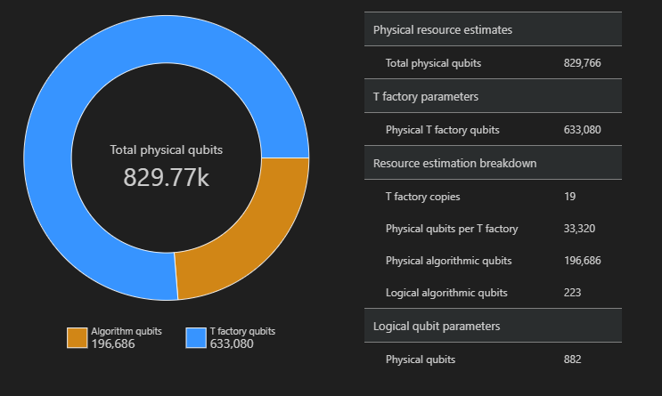
SpaceChart(result)
이 예제에서는 알고리즘을 실행하는 데 필요한 실제 큐비트 수가 829766 196686 알고리즘 큐비트이고 그 중 633080은 T 팩터리 큐비트입니다.
기본값 변경 및 알고리즘 예측
프로그램에 대한 리소스 예측 요청을 제출할 때 필요에 따라 몇 가지 매개 변수를 지정할 수 있습니다. 필드를 jobParams 사용하여 작업 실행에 전달할 수 있는 모든 target 매개 변수에 액세스하고 어떤 기본값이 가정되었는지 확인합니다.
result['jobParams']
{'errorBudget': 0.001,
 'qecScheme': {'crossingPrefactor': 0.03,
  'errorCorrectionThreshold': 0.01,
  'logicalCycleTime': '(4 * twoQubitGateTime + 2 * oneQubitMeasurementTime) * codeDistance',
  'name': 'surface_code',
  'physicalQubitsPerLogicalQubit': '2 * codeDistance * codeDistance'},
 'qubitParams': {'instructionSet': 'GateBased',
  'name': 'qubit_gate_ns_e3',
  'oneQubitGateErrorRate': 0.001,
  'oneQubitGateTime': '50 ns',
  'oneQubitMeasurementErrorRate': 0.001,
  'oneQubitMeasurementTime': '100 ns',
  'tGateErrorRate': 0.001,
  'tGateTime': '50 ns',
  'twoQubitGateErrorRate': 0.001,
  'twoQubitGateTime': '50 ns'}}
Resource Estimator에서 qubit_gate_ns_e3 큐비트 모델, surface_code 오류 수정 코드 및 0.001 오류 예산을 예측의 기본값으로 사용하는 것을 볼 수 있습니다.
사용자 지정할 수 있는 매개 변수는 다음과 같습니다 target .
errorBudget- 알고리즘에 대해 허용되는 전체 오류 예산qecScheme- QEC(양자 오류 수정) 체계qubitParams- 물리적 큐비트 매개 변수constraints- 구성 요소 수준의 제약 조건distillationUnitSpecifications- T 팩터리 증류 알고리즘에 대한 사양estimateType- 단일 또는 프론티어
자세한 내용은 리소스 예측 도구에 대한 대상 매개 변수를 참조하세요.
큐비트 모델 변경
Majorana 기반 큐비트 매개 변수 qubitParams인 "qubit_maj_ns_e6"을 사용하여 동일한 알고리즘에 대한 비용을 예측할 수 있습니다.
result_maj = qsharp.estimate("RunProgram()", params={
                "qubitParams": {
                    "name": "qubit_maj_ns_e6"
                }})
EstimateDetails(result_maj)
양자 오류 수정 체계 변경
Floquet QEC 체계 qecScheme을 사용하여 Majorana 기반 큐비트 매개 변수에서 동일한 예에 대한 리소스 예측 작업을 다시 실행할 수 있습니다.
result_maj = qsharp.estimate("RunProgram()", params={
                "qubitParams": {
                    "name": "qubit_maj_ns_e6"
                },
                "qecScheme": {
                    "name": "floquet_code"
                }})
EstimateDetails(result_maj)
오류 예산 변경
다음으로 errorBudget 10%로 동일한 양자 회로를 다시 실행합니다.
result_maj = qsharp.estimate("RunProgram()", params={
                "qubitParams": {
                    "name": "qubit_maj_ns_e6"
                },
                "qecScheme": {
                    "name": "floquet_code"
                },
                "errorBudget": 0.1})
EstimateDetails(result_maj)
리소스 추정기를 사용하여 일괄 처리
Azure Quantum 리소스 추정기를 사용하면 여러 매개 변수 구성 target 을 실행하고 결과를 비교할 수 있습니다. 이러한 기능은 다양한 큐비트 모델의 비용, QEC 스키마 또는 오류 예산을 비교하려는 경우에 유용합니다.
매개 변수 목록을 함수의 target 매개 변수에 전달하여 일괄 처리 추정을
paramsqsharp.estimate수행할 수 있습니다. 예를 들어 기본 매개 변수와 Floquet QEC 스키마를 사용하여 Majorana 기반 큐비트 매개 변수를 사용하여 동일한 알고리즘을 실행합니다.result_batch = qsharp.estimate("RunProgram()", params= [{}, # Default parameters { "qubitParams": { "name": "qubit_maj_ns_e6" }, "qecScheme": { "name": "floquet_code" } }]) result_batch.summary_data_frame(labels=["Gate-based ns, 10⁻³", "Majorana ns, 10⁻⁶"])모델 논리 큐비트 논리 깊이 T 상태 코드 거리 T 팩터리 T 팩터리 분수 물리적 큐비트 rQOPS 물리적 런타임 게이트 기반 ns, 10⁻³ 223 3.64M 4.70M 21 19 76.30 % 829.77k 26.55M 31초 Majorana ns, 10⁻⁶ 223 3.64M 4.70M 5 19 63.02 % 79.60k 148.67M 5초 클래스를 사용하여 추정 매개 변수 목록을 생성할
EstimatorParams수도 있습니다.from qsharp.estimator import EstimatorParams, QubitParams, QECScheme, LogicalCounts labels = ["Gate-based µs, 10⁻³", "Gate-based µs, 10⁻⁴", "Gate-based ns, 10⁻³", "Gate-based ns, 10⁻⁴", "Majorana ns, 10⁻⁴", "Majorana ns, 10⁻⁶"] params = EstimatorParams(num_items=6) params.error_budget = 0.333 params.items[0].qubit_params.name = QubitParams.GATE_US_E3 params.items[1].qubit_params.name = QubitParams.GATE_US_E4 params.items[2].qubit_params.name = QubitParams.GATE_NS_E3 params.items[3].qubit_params.name = QubitParams.GATE_NS_E4 params.items[4].qubit_params.name = QubitParams.MAJ_NS_E4 params.items[4].qec_scheme.name = QECScheme.FLOQUET_CODE params.items[5].qubit_params.name = QubitParams.MAJ_NS_E6 params.items[5].qec_scheme.name = QECScheme.FLOQUET_CODEqsharp.estimate("RunProgram()", params=params).summary_data_frame(labels=labels)모델 논리 큐비트 논리 깊이 T 상태 코드 거리 T 팩터리 T 팩터리 분수 물리적 큐비트 rQOPS 물리적 런타임 게이트 기반 μs, 10⁻5 223 3.64M 4.70M 17 13 40.54% 216.77k 21.86k 10시간 게이트 기반 µs, 10⁻⁴ 223 3.64M 4.70M 9 14 43.17% 63.57k 41.30k 5시간 게이트 기반 ns, 10⁻³ 223 3.64M 4.70M 17 16 69.08% 416.89k 32.79M 25초 게이트 기반 ns, 10⁻⁴ 223 3.64M 4.70M 9 14 43.17% 63.57k 61.94M 13초 Majorana ns, 10⁻⁴ 223 3.64M 4.70M 9 19 82.75% 501.48k 82.59M 10초 Majorana ns, 10⁻⁶ 223 3.64M 4.70M 5 13 31.47% 42.96k 148.67M 5초
파레토 프론티어 예측 실행
알고리즘의 리소스를 추정할 때는 실제 큐비트 수와 알고리즘의 런타임 간의 절충을 고려해야 합니다. 알고리즘의 런타임을 줄이기 위해 가능한 한 많은 실제 큐비트를 할당하는 것을 고려할 수 있습니다. 그러나 물리적 큐비트의 수는 양자 하드웨어에서 사용할 수 있는 물리적 큐비트의 수로 제한됩니다.
Pareto 프론티어 예측은 동일한 알고리즘에 대한 여러 예상치를 제공하며, 각각 큐비트 수와 런타임 간의 장단점이 있습니다.
Pareto 프론티어 추정을 사용하여 리소스 추정기를 실행하려면 매개 변수를
"estimateType"target .로"frontier"지정해야 합니다. 예를 들어 Pareto 프론티어 추정을 사용하여 표면 코드를 사용하여 Majorana 기반 큐비트 매개 변수를 사용하여 동일한 알고리즘을 실행합니다.result = qsharp.estimate("RunProgram()", params= {"qubitParams": { "name": "qubit_maj_ns_e4" }, "qecScheme": { "name": "surface_code" }, "estimateType": "frontier", # frontier estimation } )이 함수를
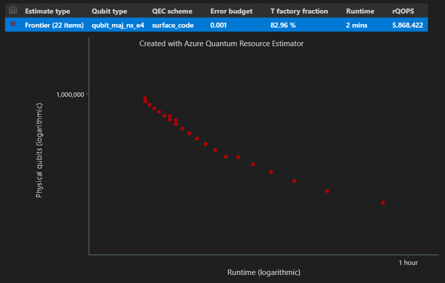
EstimatesOverview사용하여 전체 실제 리소스 수가 포함된 테이블을 표시할 수 있습니다. 첫 번째 행 옆의 아이콘을 클릭하여 표시할 열을 선택합니다. 실행 이름, 예측 형식, 큐비트 유형, qec 체계, 오류 예산, 논리 큐비트, 논리 깊이, 코드 거리, T 상태, T 팩터리, T 팩터리 분수, 런타임, rQOPS 및 실제 큐비트 중에서 선택할 수 있습니다.from qsharp_widgets import EstimatesOverview EstimatesOverview(result)
결과 테이블의 추정 형식 열에서 알고리즘에 대한 {큐비트 수, 런타임}의 다양한 조합 수를 볼 수 있습니다. 이 경우 리소스 추정기는 수천 가지 가능한 조합 중에서 22가지 최적의 조합을 찾습니다.
시공간 다이어그램
이 함수는 EstimatesOverview 리소스 추정기의 시공간 다이어그램 도 표시합니다.
시공간 다이어그램은 각 {큐비트 수, 런타임} 쌍에 대한 알고리즘의 실제 큐비트 수와 런타임을 보여 줍니다. 각 지점을 마우스로 가리키면 해당 시점에서 리소스 예측의 세부 정보를 볼 수 있습니다.
파레토 프론티어 추정을 사용하여 일괄 처리
여러 매개 변수 구성을 target 예측하고 비교하려면 매개 변수를 추가
"estimateType": "frontier",합니다.result = qsharp.estimate( "RunProgram()", [ { "qubitParams": { "name": "qubit_maj_ns_e4" }, "qecScheme": { "name": "surface_code" }, "estimateType": "frontier", # Pareto frontier estimation }, { "qubitParams": { "name": "qubit_maj_ns_e6" }, "qecScheme": { "name": "floquet_code" }, "estimateType": "frontier", # Pareto frontier estimation }, ] ) EstimatesOverview(result, colors=["#1f77b4", "#ff7f0e"], runNames=["e4 Surface Code", "e6 Floquet Code"])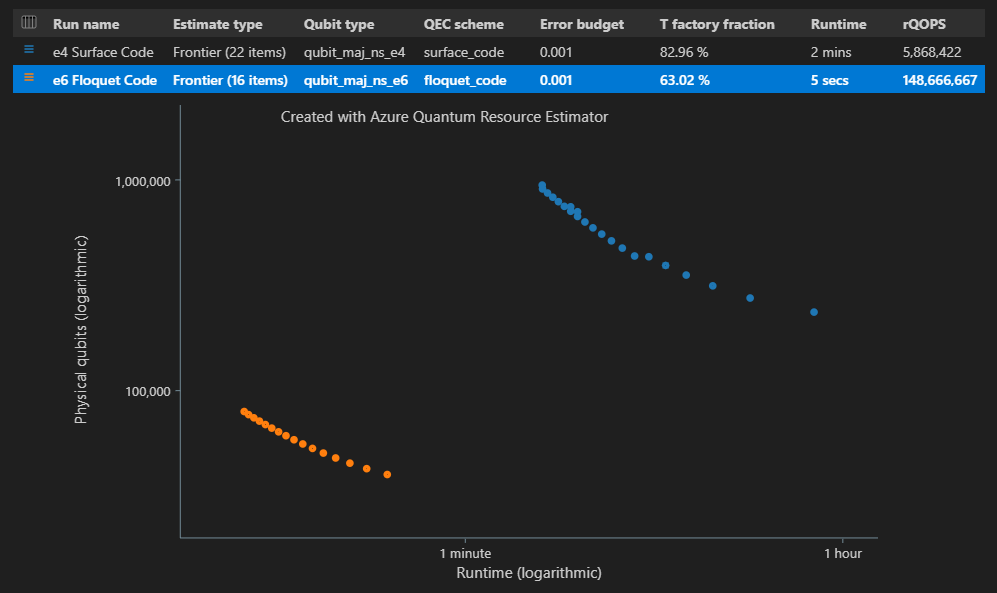
참고 항목
함수를 사용하여
EstimatesOverview큐비트 시간 다이어그램의 색을 정의하고 이름을 실행할 수 있습니다.Pareto 프론티어 추정을 사용하여 여러 매개 변수 구성 target 을 실행하는 경우 각 {큐비트 수, 런타임} 쌍에 해당하는 시공간 다이어그램의 특정 지점에 대한 리소스 예상치를 볼 수 있습니다. 예를 들어 다음 코드는 두 번째(추정 인덱스=0) 실행 및 네 번째(지점 인덱스=3) 최단 런타임에 대한 예상 세부 정보 사용량을 보여 줍니다.
EstimateDetails(result[1], 4)시공간 다이어그램의 특정 지점에 대한 공간 다이어그램을 볼 수도 있습니다. 예를 들어 다음 코드는 조합의 첫 번째 실행(인덱스=0 추정) 및 세 번째로 짧은 런타임(점 인덱스=2)에 대한 공간 다이어그램을 보여 줍니다.
SpaceChart(result[0], 2)
Qiskit의 필수 구성 요소
- 활성 구독이 있는 Azure 계정. Azure 계정이 없는 경우 무료로 등록하고 종량제 구독에 등록합니다.
- Azure Quantum 작업 영역 자세한 내용은 Azure Quantum 작업 영역 만들기를 참조하세요.
작업 영역에서 Azure Quantum 리소스 추정기 target 사용
리소스 추정기는 target Microsoft Quantum 컴퓨팅 공급자입니다. 리소스 예측 도구 릴리스 이후 작업 영역을 만든 경우 Microsoft Quantum Computing 공급자가 작업 영역에 자동으로 추가되었습니다.
기존 Azure Quantum 작업 영역을 사용하는 경우:
- Azure Portal에서 작업 영역을 엽니다.
- 왼쪽 패널의 작업에서 공급자를 선택합니다.
- + 공급자 추가를 선택합니다.
- Microsoft Quantum Computing에 대해 + 추가를 선택합니다.
- 학습 및 개발을 선택하고 추가를 선택합니다.
작업 영역에서 새 Notebook 만들기
- Azure Portal에 로그인하고 Azure Quantum 작업 영역을 선택합니다.
- 작업에서 Notebook을 선택합니다.
- 내 전자 필기장을 클릭하고 새로 추가를 클릭합니다.
- 커널 형식에서 IPython을 선택합니다.
- 파일의 이름을 입력하고 파일 만들기를 클릭합니다.
새 Notebook이 열리면 구독 및 작업 영역 정보에 따라 첫 번째 셀에 대한 코드가 자동으로 만들어집니다.
from azure.quantum import Workspace
workspace = Workspace (
    resource_id = "", # Your resource_id
    location = ""  # Your workspace location (for example, "westus")
)
참고 항목
달리 명시되지 않는 한 컴파일 문제를 방지하기 위해 셀을 만들 때 각 셀을 순서대로 실행해야 합니다.
셀 왼쪽의 삼각형 "재생" 아이콘을 클릭하여 코드를 실행합니다.
필요한 가져오기 로드
먼저 azure-quantum 및 qiskit.에서 추가 모듈을 가져와야 합니다.
+ 코드를 클릭하여 새 셀을 추가하고, 다음 코드를 추가하여 실행합니다.
from azure.quantum.qiskit import AzureQuantumProvider
from qiskit import QuantumCircuit, transpile
from qiskit.circuit.library import RGQFTMultiplier
Azure Quantum 서비스에 연결
다음으로, 이전 셀의 workspace 개체를 사용하여 Azure Quantum 작업 영역에 연결하는 AzureQuantumProvider 개체를 만듭니다. 백 엔드 인스턴스를 만들고 리소스 추정기를 사용자 target로 설정합니다.
provider = AzureQuantumProvider(workspace)
backend = provider.get_backend('microsoft.estimator')
양자 알고리즘 생성
이 예제에서는 양자 푸리에 변환을 사용하여 산술을 구현하는 Ruiz-Perez 및 Garcia-Escartin(arXiv:1411.5949)에 제시된 생성을 기반으로 승수에 대한 양자 회로를 만듭니다.
변수를 변경 bitwidth 하여 승수의 크기를 조정할 수 있습니다. 회로 생성은 승수 값으로 호출할 수 있는 함수에 bitwidth 래핑됩니다. 작업에는 지정된 크기의 두 개의 입력 레지스터와 지정된 bitwidth크기의 두 배 bitwidth인 하나의 출력 레지스터가 있습니다. 또한 이 함수는 양자 회로에서 직접 추출된 승수에 대한 몇 가지 논리 리소스 수를 출력합니다.
def create_algorithm(bitwidth):
    print(f"[INFO] Create a QFT-based multiplier with bitwidth {bitwidth}")

    # Print a warning for large bitwidths that will require some time to generate and
    # transpile the circuit.
    if bitwidth > 18:
        print(f"[WARN] It will take more than one minute generate a quantum circuit with a bitwidth larger than 18")

    circ = RGQFTMultiplier(num_state_qubits=bitwidth, num_result_qubits=2 * bitwidth)

    # One could further reduce the resource estimates by increasing the optimization_level,
    # however, this will also increase the runtime to construct the algorithm.  Note, that
    # it does not affect the runtime for resource estimation.
    print(f"[INFO] Decompose circuit into intrinsic quantum operations")

    circ = transpile(circ, basis_gates=SUPPORTED_INSTRUCTIONS, optimization_level=0)

    # print some statistics
    print(f"[INFO]   qubit count: {circ.num_qubits}")
    print("[INFO]   gate counts")
    for gate, count in circ.count_ops().items():
        print(f"[INFO]   - {gate}: {count}")

    return circ
참고 항목
T 상태가 없지만 측정값이 하나 이상 있는 알고리즘에 대한 실제 리소스 예측 작업을 제출할 수 있습니다.
양자 알고리즘 예측
함수를 사용하여 알고리즘의 인스턴스를 만듭니다 create_algorithm . 변수를 변경 bitwidth 하여 승수의 크기를 조정할 수 있습니다.
bitwidth = 4

circ = create_algorithm(bitwidth)
기본 가정을 사용하여 이 작업의 실제 리소스를 예측합니다. 이 메서드를 사용하여 run 회로를 Resource Estimator 백 엔드에 제출한 다음 실행 job.result() 하여 작업이 완료되고 결과를 반환할 때까지 기다릴 수 있습니다.
job = backend.run(circ)
result = job.result()
result
이렇게 하면 전체 실제 리소스 수를 보여 주는 테이블이 만들어집니다. 더 많은 정보가 있는 그룹을 축소해 비용 세부 정보를 검사할 수 있습니다.
팁
더 간결한 버전의 출력 테이블을 보려면 result.summary를 사용할 수 있습니다.
예를 들어 논리 큐비트 매개 변수 그룹을 축소하면 오류 수정 코드 거리가 15임을 더 쉽게 확인할 수 있습니다.
| 논리적 큐비트 매개 변수 | 값 |
|---|---|
| QEC 체계 | surface_code |
| 코드 거리 | 15 |
| 물리적 큐비트 | 450 |
| 논리적 주기 시간 | 6us |
| 논리적 큐비트 오류율 | 3.00E-10 |
| 교차 전인자 | 0.03 |
| 오류 수정 임계값 | 0.01 |
| 논리적 주기 시간 수식 | (4 * twoQubitGateTime + 2 * oneQubitMeasurementTime) * codeDistance |
| 물리적 큐비트 수식 | 2 * codeDistance * codeDistance |
실제 큐비트 매개 변수 그룹에서 이 추정에 대해 가정된 실제 큐비트 속성을 볼 수 있습니다. 예를 들어 단일 큐비트 측정 및 단일 큐비트 게이트를 수행하는 시간이 각각 100ns 및 50ns로 가정됩니다.
팁
result.data() 메서드를 사용하여 리소스 추정기의 출력을 Python 사전으로 액세스할 수도 있습니다.
자세한 내용은 리소스 예측 도구에 대한 출력 데이터의 전체 목록을 참조하세요.
공간 다이어그램
알고리즘 및 T 팩터리에 사용되는 실제 큐비트의 분포는 알고리즘 디자인에 영향을 미칠 수 있는 요소입니다. 이 분포를 시각화하여 알고리즘의 예상 공간 요구 사항을 더 잘 이해할 수 있습니다.
result.diagram.space
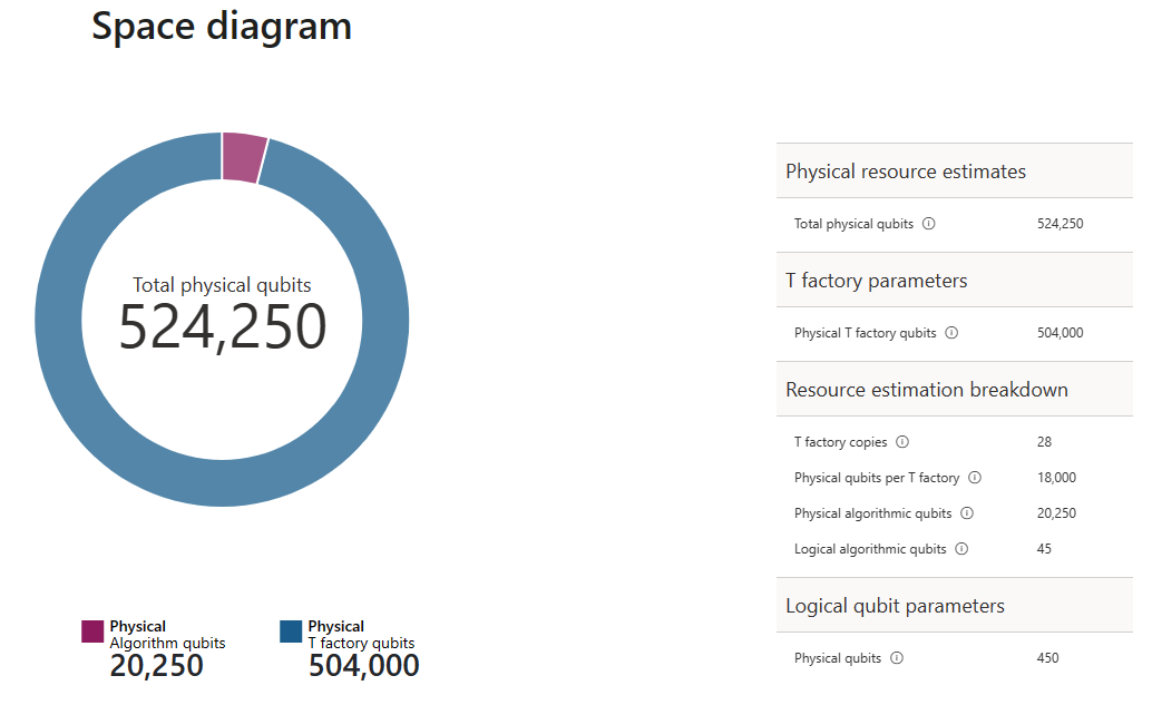
공간 다이어그램은 알고리즘 큐비트와 T 팩터리 큐비트의 비율을 보여 줍니다. T 팩터리 복사본 수(28개)는 T 팩터리의 실제 큐비트 수를 $\text{Tfactory} \cdot \text{physical qubit per T factory}= 28 \cdot 18,000 = 504,000$로 지정합니다.
자세한 내용은 T 팩터리 물리적 추정을 참조 하세요.
기본값 변경 및 알고리즘 예측
프로그램에 대한 리소스 예측 요청을 제출할 때 필요에 따라 몇 가지 매개 변수를 지정할 수 있습니다. 필드를 jobParams 사용하여 작업 실행에 전달할 수 있는 모든 값에 액세스하고 어떤 기본값이 가정되었는지 확인합니다.
result.data()["jobParams"]
{'errorBudget': 0.001,
 'qecScheme': {'crossingPrefactor': 0.03,
  'errorCorrectionThreshold': 0.01,
  'logicalCycleTime': '(4 * twoQubitGateTime + 2 * oneQubitMeasurementTime) * codeDistance',
  'name': 'surface_code',
  'physicalQubitsPerLogicalQubit': '2 * codeDistance * codeDistance'},
 'qubitParams': {'instructionSet': 'GateBased',
  'name': 'qubit_gate_ns_e3',
  'oneQubitGateErrorRate': 0.001,
  'oneQubitGateTime': '50 ns',
  'oneQubitMeasurementErrorRate': 0.001,
  'oneQubitMeasurementTime': '100 ns',
  'tGateErrorRate': 0.001,
  'tGateTime': '50 ns',
  'twoQubitGateErrorRate': 0.001,
  'twoQubitGateTime': '50 ns'}}
사용자 지정할 수 있는 매개 변수는 다음과 같습니다 target .
errorBudget- 허용되는 전체 오류 예산qecScheme- QEC(양자 오류 수정) 체계qubitParams- 물리적 큐비트 매개 변수constraints- 구성 요소 수준의 제약 조건distillationUnitSpecifications- T 팩터리 증류 알고리즘에 대한 사양
자세한 내용은 리소스 예측 도구에 대한 대상 매개 변수를 참조하세요.
큐비트 모델 변경
다음으로 Majorana 기반 큐비트 매개 변수를 사용하여 동일한 알고리즘에 대한 비용을 예측합니다. qubit_maj_ns_e6
job = backend.run(circ,
    qubitParams={
        "name": "qubit_maj_ns_e6"
    })
result = job.result()
result
물리적 개수를 프로그래밍 방식으로 검사할 수 있습니다. 예를 들어 알고리즘을 실행하기 위해 만든 T 팩터리에 대한 세부 정보를 탐색할 수 있습니다.
result.data()["tfactory"]
{'eccDistancePerRound': [1, 1, 5],
 'logicalErrorRate': 1.6833177305222897e-10,
 'moduleNamePerRound': ['15-to-1 space efficient physical',
  '15-to-1 RM prep physical',
  '15-to-1 RM prep logical'],
 'numInputTstates': 20520,
 'numModulesPerRound': [1368, 20, 1],
 'numRounds': 3,
 'numTstates': 1,
 'physicalQubits': 16416,
 'physicalQubitsPerRound': [12, 31, 1550],
 'runtime': 116900.0,
 'runtimePerRound': [4500.0, 2400.0, 110000.0]}
참고 항목
기본적으로 런타임은 나노초로 표시됩니다.
이 데이터를 사용하여 T 팩터리에서 필요한 T 상태를 생성하는 방법에 대한 몇 가지 설명을 생성할 수 있습니다.
data = result.data()
tfactory = data["tfactory"]
breakdown = data["physicalCounts"]["breakdown"]
producedTstates = breakdown["numTfactories"] * breakdown["numTfactoryRuns"] * tfactory["numTstates"]

print(f"""A single T factory produces {tfactory["logicalErrorRate"]:.2e} T states with an error rate of (required T state error rate is {breakdown["requiredLogicalTstateErrorRate"]:.2e}).""")
print(f"""{breakdown["numTfactories"]} copie(s) of a T factory are executed {breakdown["numTfactoryRuns"]} time(s) to produce {producedTstates} T states ({breakdown["numTstates"]} are required by the algorithm).""")
print(f"""A single T factory is composed of {tfactory["numRounds"]} rounds of distillation:""")
for round in range(tfactory["numRounds"]):
    print(f"""- {tfactory["numModulesPerRound"][round]} {tfactory["moduleNamePerRound"][round]} unit(s)""")
A single T factory produces 1.68e-10 T states with an error rate of (required T state error rate is 2.77e-08).
23 copies of a T factory are executed 523 time(s) to produce 12029 T states (12017 are required by the algorithm).
A single T factory is composed of 3 rounds of distillation:
- 1368 15-to-1 space efficient physical unit(s)
- 20 15-to-1 RM prep physical unit(s)
- 1 15-to-1 RM prep logical unit(s)
양자 오류 수정 체계 변경
이제 Floqued QEC 스키마 qecScheme를 사용하여 Majorana 기반 큐비트 매개 변수에서 동일한 예제에 대한 리소스 예측 작업을 다시 실행합니다.
job = backend.run(circ,
    qubitParams={
        "name": "qubit_maj_ns_e6"
    },
    qecScheme={
        "name": "floquet_code"
    })
result_maj_floquet = job.result()
result_maj_floquet
오류 예산 변경
10%의 동일한 양자 회로를 errorBudget 다시 실행해 보겠습니다.
job = backend.run(circ,
    qubitParams={
        "name": "qubit_maj_ns_e6"
    },
    qecScheme={
        "name": "floquet_code"
    },
    errorBudget=0.1)
result_maj_floquet_e1 = job.result()
result_maj_floquet_e1
참고 항목
리소스 예측 도구로 작업하는 동안 문제가 발생하는 경우 문제 해결 페이지를 확인하거나 문의하세요AzureQuantumInfo@microsoft.com.