자습서: 컴퓨터 오류 감지 모델 만들기, 평가 및 점수 매기기
이 자습서에서는 Microsoft Fabric에서 Synapse 데이터 과학 워크플로의 엔드 투 엔드 예제를 제공합니다. 이 시나리오에서는 기계 학습을 사용하여 오류 진단에 대한 보다 체계적인 접근 방식을 사용하고, 문제를 사전에 식별하고, 실제 머신 오류 전에 조치를 취합니다. 목표는 프로세스 온도, 회전 속도 등에 따라 컴퓨터에서 오류가 발생하는지 여부를 예측하는 것입니다.
이 자습서에서는 다음 단계를 설명합니다.
- 사용자 지정 라이브러리 설치
- 데이터 로드 및 처리
- 예비 데이터 분석을 통해 데이터 이해
- scikit-learn, LightGBM 및 MLflow를 사용하여 기계 학습 모델을 학습하고 패브릭 자동 로깅 기능을 사용하여 실험을 추적합니다.
- 패브릭
PREDICT기능을 사용하여 학습된 모델의 점수를 매기고, 최상의 모델을 저장하고, 해당 모델을 로드하여 예측합니다. - Power BI 시각화를 사용하여 로드된 모델 성능 표시
필수 조건
Microsoft Fabric 구독을 가져옵니다. 또는 무료 Microsoft Fabric 평가판에 등록합니다.
Microsoft Fabric에 로그인합니다.
홈페이지 왼쪽의 환경 전환기를 사용하여 Synapse 데이터 과학 환경으로 전환합니다.
- 필요한 경우 Microsoft Fabric에서 레이크하우스 만들기에 설명된 대로 Microsoft Fabric 레이크하우스를 만듭니다.
전자 필기장에서 팔로우
다음 옵션 중 하나를 선택하여 전자 필기장에서 따를 수 있습니다.
- 데이터 과학 환경에서 기본 제공 Notebook 열기 및 실행
- GitHub에서 데이터 과학 환경으로 Notebook 업로드
기본 제공 Notebook 열기
샘플 컴퓨터 오류 Notebook은 이 자습서와 함께 제공됩니다.
Synapse 데이터 과학 환경에서 자습서의 기본 제공 샘플 Notebook을 열려면 다음을 수행합니다.
Synapse 데이터 과학 홈페이지로 이동합니다.
샘플 사용을 선택합니다.
해당 샘플을 선택합니다.
- 기본 Python(엔드 투 엔드 워크플로) 탭에서 샘플이 Python 자습서용인 경우
- R(엔드 투 엔드 워크플로) 탭에서 샘플이 R 자습서용인 경우
- 빠른 자습서 탭에서 샘플이 빠른 자습서용인 경우
코드 실행을 시작하기 전에 Lakehouse를 Notebook 에 연결합니다.
GitHub에서 Notebook 가져오기
AISample - 예측 유지 관리 Notebook은 이 자습서와 함께 제공됩니다.
이 자습서에 대해 함께 제공되는 Notebook을 열려면 데이터 과학 자습서를 위해 시스템 준비 자습서의 지침에 따라 Notebook을 작업 영역으로 가져옵니다.
이 페이지에서 코드를 복사하여 붙여 넣으면 새 Notebook을 만들 수 있습니다.
코드 실행을 시작하기 전에 Lakehouse를 Notebook에 연결해야 합니다.
1단계: 사용자 지정 라이브러리 설치
기계 학습 모델 개발 또는 임시 데이터 분석의 경우 Apache Spark 세션에 대한 사용자 지정 라이브러리를 신속하게 설치해야 할 수 있습니다. 라이브러리를 설치하는 두 가지 옵션이 있습니다.
- 현재 Notebook에만 라이브러리를 설치하려면 Notebook의 인라인 설치 기능(
%pip또는%conda)을 사용합니다. - 또는 패브릭 환경을 만들거나, 공용 원본에서 라이브러리를 설치하거나, 사용자 지정 라이브러리를 업로드한 다음, 작업 영역 관리자가 작업 영역의 기본값으로 환경을 연결할 수 있습니다. 그러면 환경의 모든 라이브러리를 작업 영역의 모든 Notebook 및 Spark 작업 정의에서 사용할 수 있게 됩니다. 환경에 대한 자세한 내용은 Microsoft Fabric에서 환경 만들기, 구성 및 사용을 참조 하세요.
이 자습서에서는 Notebook에 라이브러리를 imblearn 설치하는 데 사용합니다%pip install.
참고 항목
실행 후 %pip install PySpark 커널이 다시 시작됩니다. 다른 셀을 실행하기 전에 필요한 라이브러리를 설치합니다.
# Use pip to install imblearn
%pip install imblearn
2단계: 데이터 로드
데이터 세트는 산업 설정에서 흔히 볼 수 있는 시간 함수로 제조 기계의 매개 변수 로깅을 시뮬레이션합니다. 열로 기능이 있는 행으로 저장된 10,000개의 데이터 요소로 구성됩니다. 기능은 다음과 같습니다.
1에서 10000까지의 UID(고유 식별자)
제품 품질 변형 및 변형별 일련 번호를 나타내는 문자 L(낮음), M(중간) 또는 H(높음)로 구성된 제품 ID입니다. 저품질, 중형 및 고품질 변형은 각각 모든 제품의 60%, 30%, 10%를 차지합니다.
공기 온도( 켈빈(K)
공정 온도(켈빈도)
회전 속도(분당 회전 수)(RPM)
Torque, in Newton-Meters (Nm)
도구 마모(분). 품질 변형 H, M 및 L은 프로세스에 사용되는 도구에 각각 5, 3 및 2분의 도구 마모를 추가합니다.
컴퓨터가 특정 데이터 요소에서 실패했는지 여부를 나타내는 컴퓨터 오류 레이블입니다. 이 특정 데이터 요소에는 다음과 같은 5가지 독립적인 오류 모드가 있을 수 있습니다.
- TWF(도구 착용 실패): 200분에서 240분 사이에 임의로 선택한 도구 착용 시간에 도구를 교체하거나 실패합니다.
- HDF(열 방출 실패): 온도와 프로세스 온도의 차이가 8.6K 미만이고 도구의 회전 속도가 1380 RPM 미만인 경우 열 소멸로 인해 프로세스 오류가 발생합니다.
- PWF(정전): 토크 및 회전 속도(rad/s)의 곱은 프로세스에 필요한 전력과 같습니다. 이 전원이 3,500W 이하로 떨어지거나 9,000W를 초과하면 프로세스가 실패합니다.
- OSF(OverStrain Failure): 도구 마모 및 토크 제품이 L 제품 변형의 최소 Nm 11,000을 초과하는 경우(M의 경우 12,000개, H의 경우 13,000개) 초과로 인해 프로세스가 실패합니다.
- RNF(임의 오류): 프로세스 매개 변수에 관계없이 각 프로세스의 실패 확률은 0.1%입니다.
참고 항목
위의 오류 모드 중 하나 이상이 true이면 프로세스가 실패하고 "컴퓨터 오류" 레이블이 1로 설정됩니다. 기계 학습 방법은 프로세스 실패를 발생시킨 오류 모드를 확인할 수 없습니다.
데이터 세트를 다운로드하고 레이크하우스에 업로드
Azure Open Datasets 컨테이너에 커넥트 예측 유지 관리 데이터 세트를 로드합니다. 이 코드는 공개적으로 사용 가능한 버전의 데이터 세트를 다운로드한 다음 Fabric Lakehouse에 저장합니다.
Important
실행하기 전에 Notebook에 Lakehouse를 추가합니다. 그렇지 않으면 오류가 발생합니다. 레이크하우스를 추가하는 방법에 대한 자세한 내용은 커넥트 레이크하우스 및 노트북을 참조하세요.
# Download demo data files into the lakehouse if they don't exist
import os, requests
DATA_FOLDER = "Files/predictive_maintenance/"  # Folder that contains the dataset
DATA_FILE = "predictive_maintenance.csv"  # Data file name
remote_url = "https://synapseaisolutionsa.blob.core.windows.net/public/MachineFaultDetection"
file_list = ["predictive_maintenance.csv"]
download_path = f"/lakehouse/default/{DATA_FOLDER}/raw"

if not os.path.exists("/lakehouse/default"):
    raise FileNotFoundError(
        "Default lakehouse not found, please add a lakehouse and restart the session."
    )
os.makedirs(download_path, exist_ok=True)
for fname in file_list:
    if not os.path.exists(f"{download_path}/{fname}"):
        r = requests.get(f"{remote_url}/{fname}", timeout=30)
        with open(f"{download_path}/{fname}", "wb") as f:
            f.write(r.content)
print("Downloaded demo data files into lakehouse.")
레이크하우스에 데이터 세트를 다운로드한 후 Spark 데이터 프레임으로 로드할 수 있습니다.
df = (
    spark.read.option("header", True)
    .option("inferSchema", True)
    .csv(f"{DATA_FOLDER}raw/{DATA_FILE}")
    .cache()
)
df.show(5)
이 표에는 데이터의 미리 보기가 표시됩니다.
| UDI | Product ID | 유형 | 대기 온도[K] | 프로세스 온도[K] | 회전 속도[rpm] | 토크[Nm] | 도구 마모[min] | 대상 | 오류 유형 |
|---|---|---|---|---|---|---|---|---|---|
| 1 | M14860 | M | 298.1 | 308.6 | 1551 | 42.8 | 0 | 0 | 실패 없음 |
| 2 | L47181 | L | 298.2 | 308.7 | 1408 | 46.3 | 3 | 0 | 실패 없음 |
| 3 | L47182 | L | 298.1 | 308.5 | 1498 | 49.4 | 5 | 0 | 실패 없음 |
| 4 | L47183 | L | 298.2 | 308.6 | 1433 | 39.5 | 7 | 0 | 실패 없음 |
| 5 | L47184 | L | 298.2 | 308.7 | 1408 | 40.0 | 9 | 0 | 실패 없음 |
Lakehouse 델타 테이블에 Spark DataFrame 쓰기
다음 단계에서 Spark 작업을 용이하게 하려면 데이터 형식을 지정합니다(예: 공백을 밑줄로 바꾸기).
# Replace the space in the column name with an underscore to avoid an invalid character while saving
df = df.toDF(*(c.replace(' ', '_') for c in df.columns))
table_name = "predictive_maintenance_data"
df.show(5)
이 표에서는 서식이 지정된 열 이름을 가진 데이터의 미리 보기를 보여 봅니다.
| UDI | Product_ID | Type | Air_temperature_[K] | Process_temperature_[K] | Rotational_speed_[rpm] | Torque_[Nm] | Tool_wear_[min] | 대상 | Failure_Type |
|---|---|---|---|---|---|---|---|---|---|
| 1 | M14860 | M | 298.1 | 308.6 | 1551 | 42.8 | 0 | 0 | 실패 없음 |
| 2 | L47181 | L | 298.2 | 308.7 | 1408 | 46.3 | 3 | 0 | 실패 없음 |
| 3 | L47182 | L | 298.1 | 308.5 | 1498 | 49.4 | 5 | 0 | 실패 없음 |
| 4 | L47183 | L | 298.2 | 308.6 | 1433 | 39.5 | 7 | 0 | 실패 없음 |
| 5 | L47184 | L | 298.2 | 308.7 | 1408 | 40.0 | 9 | 0 | 실패 없음 |
# Save data with processed columns to the lakehouse
df.write.mode("overwrite").format("delta").save(f"Tables/{table_name}")
print(f"Spark DataFrame saved to delta table: {table_name}")
3단계: 데이터를 전처리하고 예비 데이터 분석 수행
Pandas 호환 인기 그리기 라이브러리를 사용하도록 Spark DataFrame을 pandas DataFrame으로 변환합니다.
팁
큰 데이터 세트의 경우 해당 데이터 세트의 일부를 로드해야 할 수 있습니다.
data = spark.read.format("delta").load("Tables/predictive_maintenance_data")
SEED = 1234
df = data.toPandas()
df.drop(['UDI', 'Product_ID'],axis=1,inplace=True)
# Rename the Target column to IsFail
df = df.rename(columns = {'Target': "IsFail"})
df.info()
필요에 따라 데이터 세트의 특정 열을 부동 소수점 또는 정수 형식으로 변환하고 문자열('L', 'M', 'H')을 숫자 값(0, 1, 2)으로 매핑합니다.
# Convert temperature, rotational speed, torque, and tool wear columns to float
df['Air_temperature_[K]'] = df['Air_temperature_[K]'].astype(float)
df['Process_temperature_[K]'] = df['Process_temperature_[K]'].astype(float)
df['Rotational_speed_[rpm]'] = df['Rotational_speed_[rpm]'].astype(float)
df['Torque_[Nm]'] = df['Torque_[Nm]'].astype(float)
df['Tool_wear_[min]'] = df['Tool_wear_[min]'].astype(float)

# Convert the 'Target' column to an integer
df['IsFail'] = df['IsFail'].astype(int)
# Map 'L', 'M', 'H' to numerical values
df['Type'] = df['Type'].map({'L': 0, 'M': 1, 'H': 2})
시각화를 통해 데이터 탐색
# Import packages and set plotting style
import seaborn as sns
import matplotlib.pyplot as plt
import pandas as pd
sns.set_style('darkgrid')

# Create the correlation matrix
corr_matrix = df.corr(numeric_only=True)

# Plot a heatmap
plt.figure(figsize=(10, 8))
sns.heatmap(corr_matrix, annot=True)
plt.show()
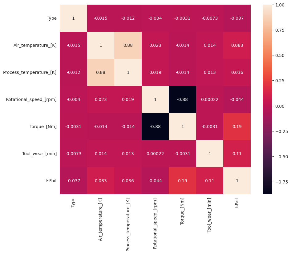
예상대로 실패()는IsFail 선택한 기능(열)과 상관 관계가 있습니다. 상관 관계 행렬은 변수와 상관 관계가 가장 높은 , Rotational_speedProcess_temperature, Torque및 Tool_wear 가장 높은 상관 관계를 IsFail 보여줍니다Air_temperature.
# Plot histograms of select features
fig, axes = plt.subplots(2, 3, figsize=(18,10))
columns = ['Air_temperature_[K]', 'Process_temperature_[K]', 'Rotational_speed_[rpm]', 'Torque_[Nm]', 'Tool_wear_[min]']
data=df.copy()
for ind, item in enumerate (columns):
    column = columns[ind]
    df_column = data[column]
    df_column.hist(ax = axes[ind%2][ind//2], bins=32).set_title(item)
fig.supylabel('count')
fig.subplots_adjust(hspace=0.2)
fig.delaxes(axes[1,2])
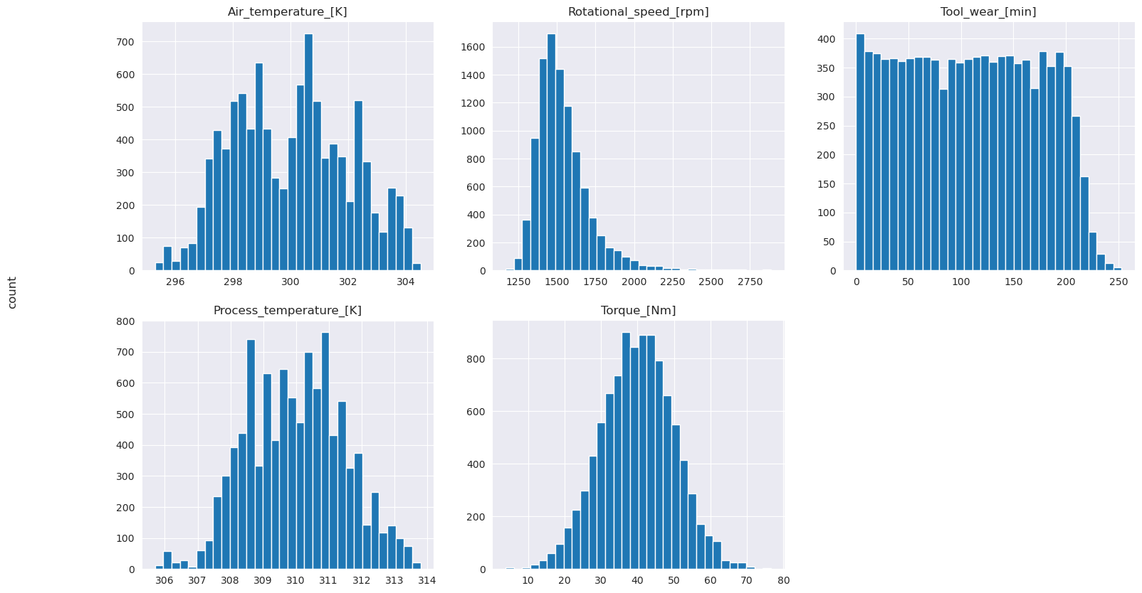
표시된 그래프에서와 같이, Air_temperature, Process_temperature, TorqueRotational_speed및 Tool_wear 변수는 스파스가 아닙니다. 기능 공간에서 연속성이 좋은 것 같습니다. 이러한 플롯은 이 데이터 세트에서 기계 학습 모델을 학습하면 새 데이터 세트로 일반화할 수 있는 신뢰할 수 있는 결과를 생성할 가능성이 있음을 확인합니다.
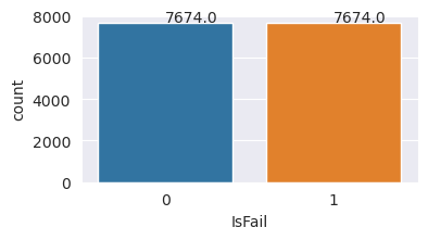
클래스 불균형에 대한 대상 변수 검사
실패 및 비일관 컴퓨터의 샘플 수를 계산하고 각 클래스에 대한 데이터 균형을 검사합니다(IsFail=0,
# Plot the counts for no failure and each failure type
plt.figure(figsize=(12, 2))
ax = sns.countplot(x='Failure_Type', data=df)
for p in ax.patches:
    ax.annotate(f'{p.get_height()}', (p.get_x()+0.4, p.get_height()+50))

plt.show()

# Plot the counts for no failure versus the sum of all failure types
plt.figure(figsize=(4, 2))
ax = sns.countplot(x='IsFail', data=df)
for p in ax.patches:
    ax.annotate(f'{p.get_height()}', (p.get_x()+0.4, p.get_height()+50))

plt.show()
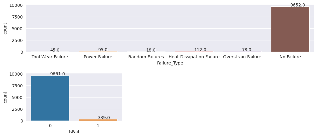
플롯은 실패하지 않는 클래스(두 번째 플롯에 표시됨 IsFail=0 )가 대부분의 샘플을 구성함을 나타냅니다. 오버샘플링 기술을 사용하여 보다 균형 잡힌 학습 데이터 세트를 만듭니다.
# Separate features and target
features = df[['Type', 'Air_temperature_[K]', 'Process_temperature_[K]', 'Rotational_speed_[rpm]', 'Torque_[Nm]', 'Tool_wear_[min]']]
labels = df['IsFail']

# Split the dataset into the training and testing sets
from sklearn.model_selection import train_test_split
X_train, X_test, y_train, y_test = train_test_split(features, labels, test_size=0.2, random_state=42)

# Ignore warnings
import warnings
warnings.filterwarnings('ignore')
# Save test data to the lakehouse for use in future sections
table_name = "predictive_maintenance_test_data"
df_test_X = spark.createDataFrame(X_test)
df_test_X.write.mode("overwrite").format("delta").save(f"Tables/{table_name}")
print(f"Spark DataFrame saved to delta table: {table_name}")
학습 데이터 세트의 클래스 균형을 조정하는 오버샘플
이전 분석 결과 데이터 세트의 불균형이 매우 높은 것으로 나타났습니다. 소수 클래스에는 모델이 의사 결정 경계를 효과적으로 학습할 수 있는 예제가 너무 적기 때문에 이러한 불균형이 문제가 됩니다.
SMOTE 는 문제를 해결할 수 있습니다. SMOTE는 합성 예제를 생성하는 널리 사용되는 오버샘플링 기술입니다. 데이터 요소 간의 유클리디안 거리를 기반으로 소수 클래스에 대한 예제를 생성합니다. 이 메서드는 소수 클래스만 복제하지 않는 새 예제를 만들기 때문에 임의 오버샘플링과 다릅니다. 이 메서드는 불균형 데이터 세트를 처리하는 보다 효과적인 기술이 됩니다.
# Disable MLflow autologging because you don't want to track SMOTE fitting
import mlflow

mlflow.autolog(disable=True)

from imblearn.combine import SMOTETomek
smt = SMOTETomek(random_state=SEED)
X_train_res, y_train_res = smt.fit_resample(X_train, y_train)

# Plot the counts for both classes
plt.figure(figsize=(4, 2))
ax = sns.countplot(x='IsFail', data=pd.DataFrame({'IsFail': y_train_res.values}))
for p in ax.patches:
    ax.annotate(f'{p.get_height()}', (p.get_x()+0.4, p.get_height()+50))

plt.show()
데이터 세트의 균형을 성공적으로 조정했습니다. 이제 모델 학습으로 이동할 수 있습니다.
4단계: 모델 학습 및 평가
MLflow 는 모델을 등록하고, 다양한 모델을 학습하고 비교하며, 예측 용도로 가장 적합한 모델을 선택합니다. 모델 학습에 다음 세 가지 모델을 사용할 수 있습니다.
- 임의 포리스트 분류자
- 로지스틱 회귀 분류자
- XGBoost 분류자
임의 포리스트 분류자 학습
import numpy as np
from sklearn.ensemble import RandomForestClassifier
from mlflow.models.signature import infer_signature
from sklearn.metrics import f1_score, accuracy_score, recall_score

mlflow.set_experiment("Machine_Failure_Classification")
mlflow.autolog(exclusive=False) # This is needed to override the preconfigured autologging behavior

with mlflow.start_run() as run:
    rfc_id = run.info.run_id
    print(f"run_id {rfc_id}, status: {run.info.status}")
    rfc = RandomForestClassifier(max_depth=5, n_estimators=50)
    rfc.fit(X_train_res, y_train_res)
    signature = infer_signature(X_train_res, y_train_res)

    mlflow.sklearn.log_model(
        rfc,
        "machine_failure_model_rf",
        signature=signature,
        registered_model_name="machine_failure_model_rf"
    )

    y_pred_train = rfc.predict(X_train)
    # Calculate the classification metrics for test data
    f1_train = f1_score(y_train, y_pred_train, average='weighted')
    accuracy_train = accuracy_score(y_train, y_pred_train)
    recall_train = recall_score(y_train, y_pred_train, average='weighted')

    # Log the classification metrics to MLflow
    mlflow.log_metric("f1_score_train", f1_train)
    mlflow.log_metric("accuracy_train", accuracy_train)
    mlflow.log_metric("recall_train", recall_train)

    # Print the run ID and the classification metrics
    print("F1 score_train:", f1_train)
    print("Accuracy_train:", accuracy_train)
    print("Recall_train:", recall_train)

    y_pred_test = rfc.predict(X_test)
    # Calculate the classification metrics for test data
    f1_test = f1_score(y_test, y_pred_test, average='weighted')
    accuracy_test = accuracy_score(y_test, y_pred_test)
    recall_test = recall_score(y_test, y_pred_test, average='weighted')

    # Log the classification metrics to MLflow
    mlflow.log_metric("f1_score_test", f1_test)
    mlflow.log_metric("accuracy_test", accuracy_test)
    mlflow.log_metric("recall_test", recall_test)

    # Print the classification metrics
    print("F1 score_test:", f1_test)
    print("Accuracy_test:", accuracy_test)
    print("Recall_test:", recall_test)
출력에서 학습 및 테스트 데이터 세트는 임의 포리스트 분류자를 사용할 때 F1 점수, 정확도 및 약 0.9의 회수를 생성합니다.
로지스틱 회귀 분류자 학습
from sklearn.linear_model import LogisticRegression

with mlflow.start_run() as run:
    lr_id = run.info.run_id
    print(f"run_id {lr_id}, status: {run.info.status}")
    lr = LogisticRegression(random_state=42)
    lr.fit(X_train_res, y_train_res)
    signature = infer_signature(X_train_res, y_train_res)

    mlflow.sklearn.log_model(
        lr,
        "machine_failure_model_lr",
        signature=signature,
        registered_model_name="machine_failure_model_lr"
    )

    y_pred_train = lr.predict(X_train)
    # Calculate the classification metrics for training data
    f1_train = f1_score(y_train, y_pred_train, average='weighted')
    accuracy_train = accuracy_score(y_train, y_pred_train)
    recall_train = recall_score(y_train, y_pred_train, average='weighted')

    # Log the classification metrics to MLflow
    mlflow.log_metric("f1_score_train", f1_train)
    mlflow.log_metric("accuracy_train", accuracy_train)
    mlflow.log_metric("recall_train", recall_train)

    # Print the run ID and the classification metrics
    print("F1 score_train:", f1_train)
    print("Accuracy_train:", accuracy_train)
    print("Recall_train:", recall_train)

    y_pred_test = lr.predict(X_test)
    # Calculate the classification metrics for test data
    f1_test = f1_score(y_test, y_pred_test, average='weighted')
    accuracy_test = accuracy_score(y_test, y_pred_test)
    recall_test = recall_score(y_test, y_pred_test, average='weighted')

    # Log the classification metrics to MLflow
    mlflow.log_metric("f1_score_test", f1_test)
    mlflow.log_metric("accuracy_test", accuracy_test)
    mlflow.log_metric("recall_test", recall_test)
XGBoost 분류자 학습
from xgboost import XGBClassifier

with mlflow.start_run() as run:
    xgb = XGBClassifier()
    xgb_id = run.info.run_id
    print(f"run_id {xgb_id}, status: {run.info.status}")
    xgb.fit(X_train_res.to_numpy(), y_train_res.to_numpy())
    signature = infer_signature(X_train_res, y_train_res)

    mlflow.xgboost.log_model(
        xgb,
        "machine_failure_model_xgb",
        signature=signature,
        registered_model_name="machine_failure_model_xgb"
    )

    y_pred_train = xgb.predict(X_train)
    # Calculate the classification metrics for training data
    f1_train = f1_score(y_train, y_pred_train, average='weighted')
    accuracy_train = accuracy_score(y_train, y_pred_train)
    recall_train = recall_score(y_train, y_pred_train, average='weighted')

    # Log the classification metrics to MLflow
    mlflow.log_metric("f1_score_train", f1_train)
    mlflow.log_metric("accuracy_train", accuracy_train)
    mlflow.log_metric("recall_train", recall_train)

    # Print the run ID and the classification metrics
    print("F1 score_train:", f1_train)
    print("Accuracy_train:", accuracy_train)
    print("Recall_train:", recall_train)

    y_pred_test = xgb.predict(X_test)
    # Calculate the classification metrics for test data
    f1_test = f1_score(y_test, y_pred_test, average='weighted')
    accuracy_test = accuracy_score(y_test, y_pred_test)
    recall_test = recall_score(y_test, y_pred_test, average='weighted')

    # Log the classification metrics to MLflow
    mlflow.log_metric("f1_score_test", f1_test)
    mlflow.log_metric("accuracy_test", accuracy_test)
    mlflow.log_metric("recall_test", recall_test)
5단계: 최상의 모델 선택 및 출력 예측
이전 섹션에서는 임의 포리스트, 로지스틱 회귀 및 XGBoost의 세 가지 분류자를 학습시켰습니다. 이제 프로그래밍 방식으로 결과에 액세스하거나 UI(사용자 인터페이스)를 사용할 수 있습니다.
UI 경로 옵션의 경우 작업 영역으로 이동하여 모델을 필터링합니다.
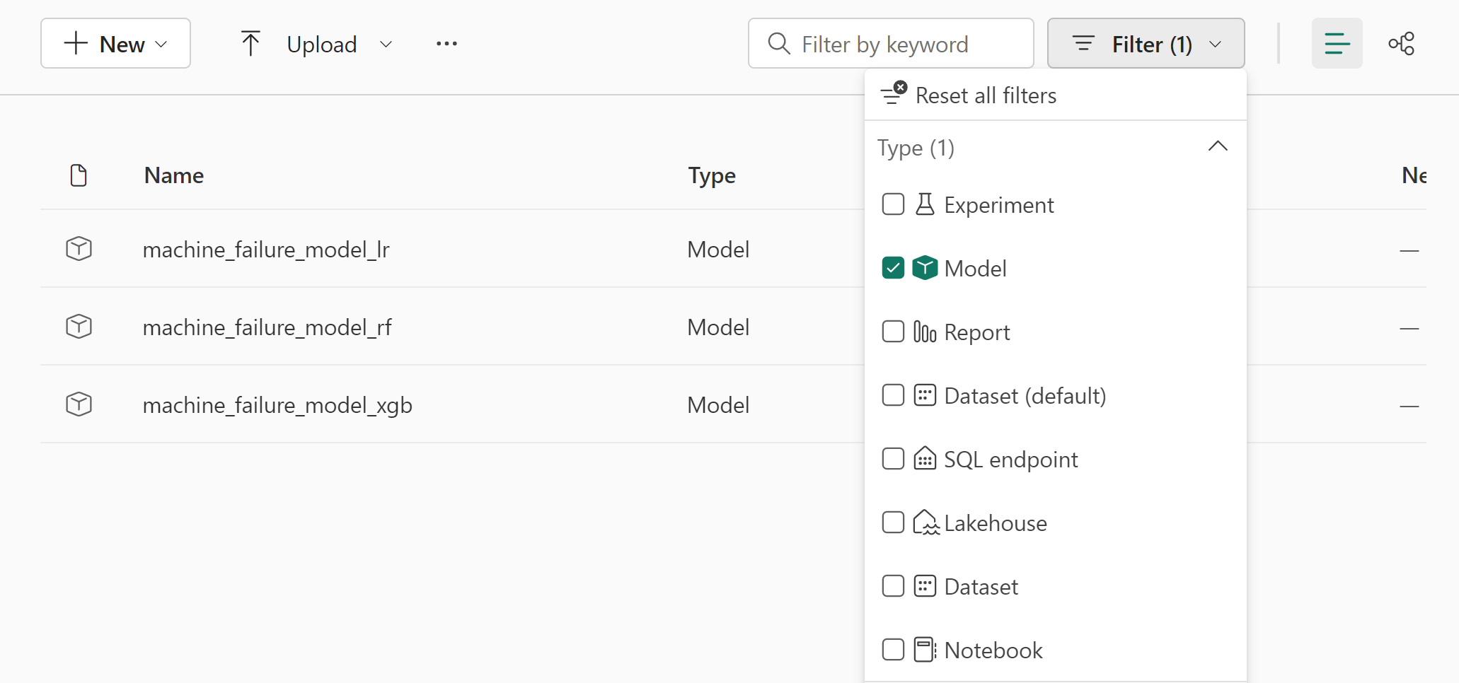
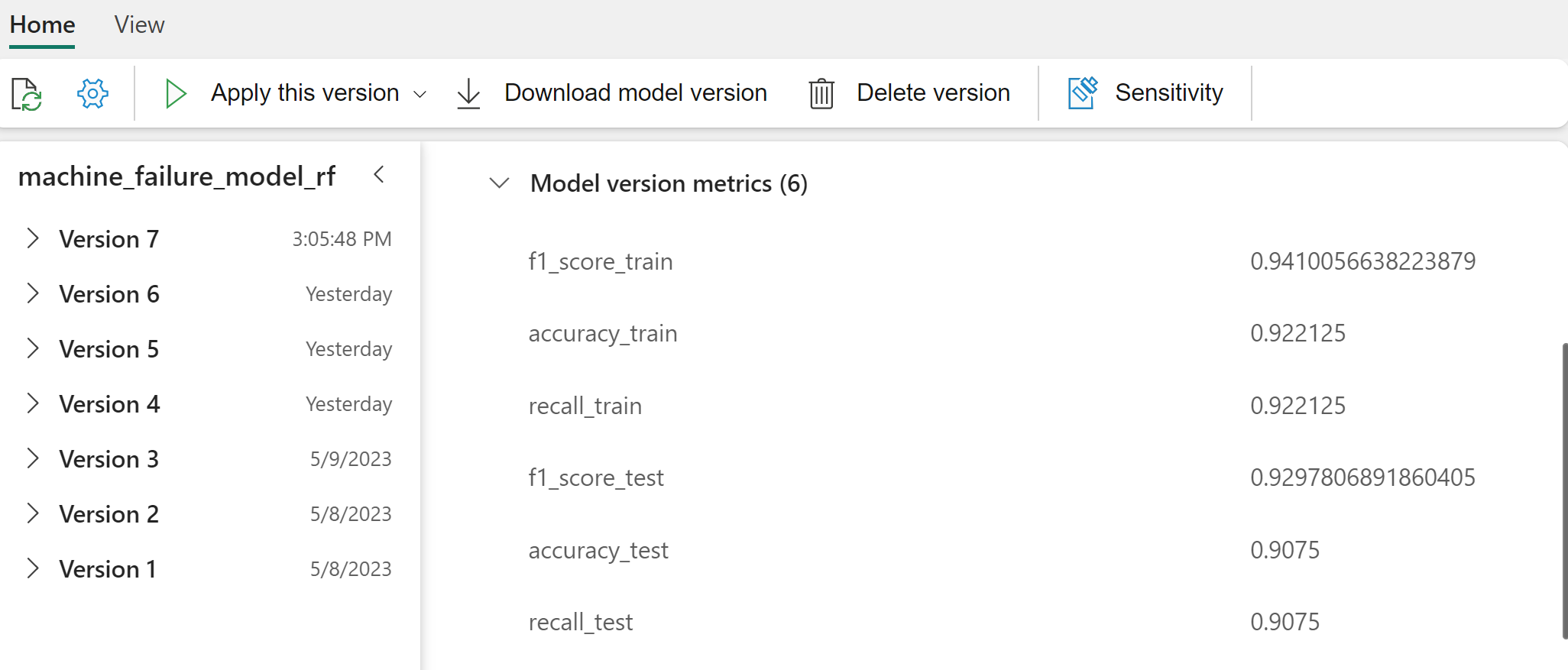
모델 성능에 대한 세부 정보를 보려면 개별 모델을 선택합니다.
이 예제에서는 MLflow를 통해 프로그래밍 방식으로 모델에 액세스하는 방법을 보여 줍니다.
runs = {'random forest classifier':   rfc_id,
        'logistic regression classifier': lr_id,
        'xgboost classifier': xgb_id}

# Create an empty DataFrame to hold the metrics
df_metrics = pd.DataFrame()

# Loop through the run IDs and retrieve the metrics for each run
for run_name, run_id in runs.items():
    metrics = mlflow.get_run(run_id).data.metrics
    metrics["run_name"] = run_name
    df_metrics = df_metrics.append(metrics, ignore_index=True)

# Print the DataFrame
print(df_metrics)
XGBoost는 학습 집합에서 최상의 결과를 생성하지만 테스트 데이터 집합에서 성능이 좋지 않습니다. 성능 저하는 과잉 맞춤을 나타냅니다. 로지스틱 회귀 분류자는 학습 및 테스트 데이터 세트 모두에서 제대로 수행되지 않습니다. 전반적으로 임의 포리스트는 학습 성능과 과잉 맞춤 방지 사이의 균형을 잘 조정합니다.
다음 섹션에서 등록된 임의 포리스트 모델을 선택하고 PREDICT 기능을 사용하여 예측을 수행합니다.
from synapse.ml.predict import MLFlowTransformer

model = MLFlowTransformer(
    inputCols=list(X_test.columns),
    outputCol='predictions',
    modelName='machine_failure_model_rf',
    modelVersion=1
)
MLFlowTransformer 추론을 위해 모델을 로드하기 위해 만든 개체를 사용하여 변환기 API를 사용하여 테스트 데이터 세트에서 모델의 점수를 매깁니다.
predictions = model.transform(spark.createDataFrame(X_test))
predictions.show()
다음 표에는 출력이 표시됩니다.
| Type | Air_temperature_[K] | Process_temperature_[K] | Rotational_speed_[rpm] | Torque_[Nm] | Tool_wear_[min] | 위한 모델 |
|---|---|---|---|---|---|---|
| 0 | 300.6 | 309.7 | 1639.0 | 30.4 | 121.0 | 0 |
| 0 | 303.9 | 313.0 | 1551.0 | 36.8 | 140.0 | 0 |
| 1 | 299.1 | 308.6 | 1491.0 | 38.5 | 166.0 | 0 |
| 0 | 300.9 | 312.1 | 1359.0 | 51.7 | 146.0 | 1 |
| 0 | 303.7 | 312.6 | 1621.0 | 38.8 | 182.0 | 0 |
| 0 | 299.0 | 310.3 | 1868.0 | 24.0 | 221.0 | 1 |
| 2 | 297.8 | 307.5 | 1631.0 | 31.3 | 124.0 | 0 |
| 0 | 297.5 | 308.2 | 1327.0 | 56.5 | 189.0 | 1 |
| 0 | 301.3 | 310.3 | 1460.0 | 41.5 | 197.0 | 0 |
| 2 | 297.6 | 309.0 | 1413.0 | 40.2 | 51.0 | 0 |
| 1 | 300.9 | 309.4 | 1724.0 | 25.6 | 119.0 | 0 |
| 0 | 303.3 | 311.3 | 1389.0 | 53.9 | 39.0 | 0 |
| 0 | 298.4 | 307.9 | 1981.0 | 23.2 | 16.0 | 0 |
| 0 | 299.3 | 308.8 | 1636.0 | 29.9 | 201.0 | 0 |
| 1 | 298.1 | 309.2 | 1460.0 | 45.8 | 80.0 | 0 |
| 0 | 300.0 | 309.5 | 1728.0 | 26.0 | 37.0 | 0 |
| 2 | 299.0 | 308.7 | 1940.0 | 19.9 | 98.0 | 0 |
| 0 | 302.2 | 310.8 | 1383.0 | 46.9 | 45.0 | 0 |
| 0 | 300.2 | 309.2 | 1431.0 | 51.3 | 57.0 | 0 |
| 0 | 299.6 | 310.2 | 1468.0 | 48.0 | 9.0 | 0 |
데이터를 레이크하우스에 저장합니다. 그런 다음 나중에 사용할 수 있는 데이터(예: Power BI 대시보드)를 사용할 수 있게 됩니다.
# Save test data to the lakehouse for use in the next section.
table_name = "predictive_maintenance_test_with_predictions"
predictions.write.mode("overwrite").format("delta").save(f"Tables/{table_name}")
print(f"Spark DataFrame saved to delta table: {table_name}")
6단계: Power BI에서 시각화를 통해 비즈니스 인텔리전스 보기
Power BI 대시보드를 사용하여 결과를 오프라인 형식으로 표시합니다.
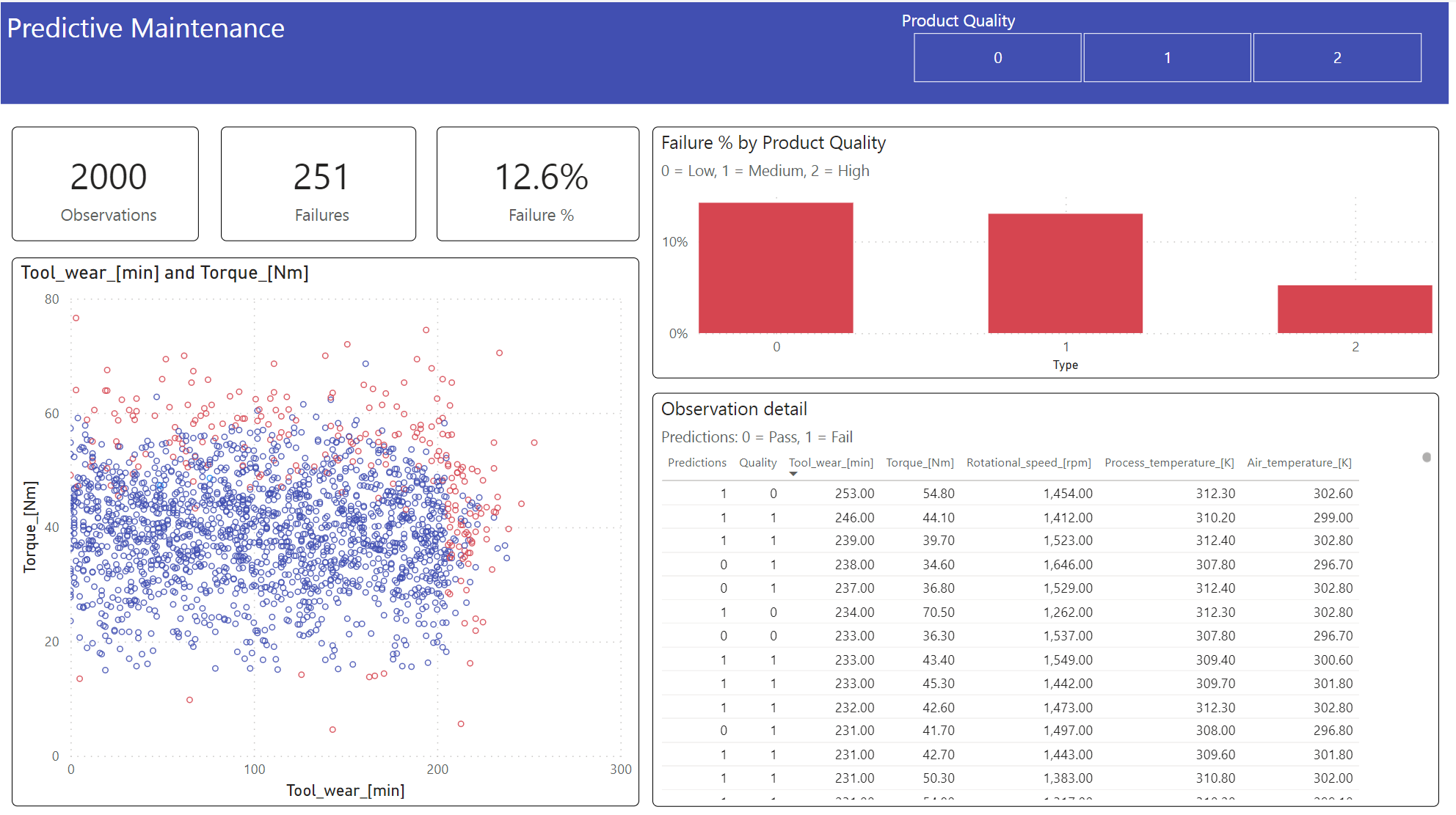
대시보드 Tool_wear Torque 는 2단계의 이전 상관 관계 분석에서 예상한 대로 실패한 사례와 완료되지 않은 사례 간에 눈에 띄는 경계를 만듭니다.