教程:创建、评估机器故障检测模型并对其评分
本教程介绍了 Microsoft Fabric 中 Synapse 数据科学工作流的端到端示例。 该方案旨在利用机器学习获得更系统的故障诊断方法,以便在机器发生实际故障之前主动识别问题并采取行动。 目标是根据过程温度、转速等特征来预测机器是否会出现故障。
本教程涵盖以下步骤:
- 安装自定义库
- 加载和处理数据
- 通过探索性数据分析了解数据
- 使用 Scikit-Learn、LightGBM、MLflow 训练机器学习模型,并使用 Fabric 自动记录功能跟踪试验
- 使用 Fabric
PREDICT功能对训练后的模型进行评分,保存最佳模型并加载该模型进行预测 - 使用 Power BI 可视化效果显示加载的模型性能
先决条件
获取 Microsoft Fabric 订阅。 或者注册免费的 Microsoft Fabric 试用版。
登录 Microsoft Fabric。
使用主页左侧的体验切换器切换到 Synapse 数据科学体验。
- 如有必要,请如在 Microsoft Fabric 中创建湖屋中所述创建 Microsoft Fabric 湖屋。
请按照笔记本进行操作
可以选择下面其中一个选项,以在笔记本中进行操作:
- 在数据科学体验中打开并运行内置笔记本
- 将笔记本从 GitHub 上传到数据科学体验
打开内置笔记本
“计算机故障”是本教程随附的示例笔记本。
要在 Synapse 数据科学体验中打开教程的内置示例笔记本,请执行以下操作:
转到 Synapse 数据科学主页。
选择“使用示例”。
选择相应的示例:
- 来自默认的“端到端工作流 (Python)”选项卡(如果示例适用于 Python 教程)。
- 来自“端到端工作流 (R)“选项卡(如果示例适用于 R 教程)。
- 从“快速教程”选项卡选择(如果示例适用于快速教程)。
从 GitHub 导入笔记本
若要打开本教程随附的笔记本,请按照让系统为数据科学做好准备教程中的说明操作,将该笔记本导入到工作区。
或者,如果要从此页面复制并粘贴代码,则可以创建新的笔记本。
在开始运行代码之前,请务必将湖屋连接到笔记本。
步骤 1:安装自定义库
对于机器学习模型开发或临时数据分析,可能需要为 Apache Spark 会话快速安装自定义库。 有两个选项可用于安装库。
- 使用笔记本的内联安装功能(
%pip或%conda),仅在当前笔记本中安装库。 - 也可以创建 Fabric 环境,安装来自公共来源的安装库或将自定义库上传到该环境,然后工作区管理员可以将环境附加为工作区的默认值。 然后,环境中的所有库都将可用于工作区中的任何笔记本和 Spark 作业定义。 有关环境的详细信息,请参阅在 Microsoft Fabric 中创建、配置和使用环境。
在本教程中,使用 %pip install 在笔记本中安装 imblearn 库。
注意
PySpark 内核将在 %pip install 之后重启。 在运行任何其他单元之前安装所需的库。
# Use pip to install imblearn
%pip install imblearn
步骤 2:加载数据
数据集模拟将制造机器的参数记录为时间函数,这在工业环境中很常见。 它由 10,000 个数据点组成,这些数据点存储为行,特征存储为列。 具体功能包括:
唯一标识符 (UID),范围从 1 到 10000
产品 ID,由字母 L(低)、M(中)或 H(高)组成,表示产品质量变体以及特定于变体的序列号。 低质量、中质量和高质量变体分别占所有产品的 60%、30% 和 10%
空气温度,以开尔文 (K) 为单位
过程温度,以开尔文为单位
转速,以转/分钟 (RPM) 为单位
扭矩,以牛顿米 (Nm) 为单位
工具磨损时间,以分钟为单位。 质量变体 H、M 和 L 分别为过程中使用的工具增加 5 分钟、3 分钟和 2 分钟的工具磨损时间。
计算机故障标签,用于指示计算机是否在特定数据点发生故障。 此特定数据点可具有以下五种独立故障模式中的任何一种:
- 工具磨损故障 (TWF):工具在随机选择的工具磨损时间(200 到 240 分钟)更换或发生故障
- 散热故障 (HDF):如果空气和古城温度之间的差异低于 8.6 K 并且工具的转速低于 1380 RPM,则散热会导致过程故障
- 电源故障 (PWF):扭矩和转速(以 rad/s 为单位)的乘积等于过程所需的功率。 如果该功率低于 3500 W 或高于 9000 W,则该过程将失败
- 过度应变故障 (OSF):如果 L 产品变体(12,000 M,13,000 H)的工具磨损时间和扭矩的乘积超过 11,000 分钟牛米,则该过程会因过度应变而失败
- 随机故障 (RNF):每个过程都有 0.1% 的几率发生故障,无论其过程参数如何
注意
如果上述故障模式中至少一种为 true,则过程将失败,并且“机器故障”标签设置为 1。 机器学习方法无法确定是哪种故障模式导致过程失败
下载数据集并上传到湖屋
连接到 Azure 开放数据集容器并加载预测性维护数据集。 以下代码将下载数据集的公开可用版本,然后将其存储在 Fabric 湖屋中:
重要
将湖屋添加到笔记本,然后才能运行该笔记本。 否则会出错。 有关添加湖屋的信息,请参阅连接湖屋和笔记本。
# Download demo data files into the lakehouse if they don't exist
import os, requests
DATA_FOLDER = "Files/predictive_maintenance/"  # Folder that contains the dataset
DATA_FILE = "predictive_maintenance.csv"  # Data file name
remote_url = "https://synapseaisolutionsa.blob.core.windows.net/public/MachineFaultDetection"
file_list = ["predictive_maintenance.csv"]
download_path = f"/lakehouse/default/{DATA_FOLDER}/raw"

if not os.path.exists("/lakehouse/default"):
    raise FileNotFoundError(
        "Default lakehouse not found, please add a lakehouse and restart the session."
    )
os.makedirs(download_path, exist_ok=True)
for fname in file_list:
    if not os.path.exists(f"{download_path}/{fname}"):
        r = requests.get(f"{remote_url}/{fname}", timeout=30)
        with open(f"{download_path}/{fname}", "wb") as f:
            f.write(r.content)
print("Downloaded demo data files into lakehouse.")
将数据集下载到湖屋后,可以将其加载为 Spark DataFrame:
df = (
    spark.read.option("header", True)
    .option("inferSchema", True)
    .csv(f"{DATA_FOLDER}raw/{DATA_FILE}")
    .cache()
)
df.show(5)
下表显示了数据的预览:
| UDI | 产品 ID | 类型 | Air temperature [K] | Process temperature [K] | Rotational speed [rpm] | Torque [Nm] | Tool wear [min] | 目标 | 失败类型 |
|---|---|---|---|---|---|---|---|---|---|
| 1 | M14860 | M | 298.1 | 308.6 | 1551 | 42.8 | 0 | 0 | 无故障 |
| 2 | L47181 | L | 298.2 | 308.7 | 1408 | 46.3 | 3 | 0 | 无故障 |
| 3 | L47182 | L | 298.1 | 308.5 | 1498 | 49.4 | 5 | 0 | 无故障 |
| 4 | L47183 | L | 298.2 | 308.6 | 1433 | 39.5 | 7 | 0 | 无故障 |
| 5 | L47184 | L | 298.2 | 308.7 | 1408 | 40.0 | 9 | 0 | 无故障 |
将 Spark DataFrame 写入湖屋增量表
设置数据格式(例如用下划线替换空格),方便后续步骤的 Spark 操作:
# Replace the space in the column name with an underscore to avoid an invalid character while saving
df = df.toDF(*(c.replace(' ', '_') for c in df.columns))
table_name = "predictive_maintenance_data"
df.show(5)
下表显示了具有重格式化列名称的数据的预览:
| UDI | Product_ID | 类型 | Air_temperature_[K] | Process_temperature_[K] | Rotational_speed_[rpm] | Torque_[Nm] | Tool_wear_[min] | 目标 | Failure_Type |
|---|---|---|---|---|---|---|---|---|---|
| 1 | M14860 | M | 298.1 | 308.6 | 1551 | 42.8 | 0 | 0 | 无故障 |
| 2 | L47181 | L | 298.2 | 308.7 | 1408 | 46.3 | 3 | 0 | 无故障 |
| 3 | L47182 | L | 298.1 | 308.5 | 1498 | 49.4 | 5 | 0 | 无故障 |
| 4 | L47183 | L | 298.2 | 308.6 | 1433 | 39.5 | 7 | 0 | 无故障 |
| 5 | L47184 | L | 298.2 | 308.7 | 1408 | 40.0 | 9 | 0 | 无故障 |
# Save data with processed columns to the lakehouse
df.write.mode("overwrite").format("delta").save(f"Tables/{table_name}")
print(f"Spark DataFrame saved to delta table: {table_name}")
步骤 3:预处理数据并执行探索性数据分析
将 Spark 数据帧转换为 Pandas 数据帧,以使用与 Pandas 兼容的常用绘图库。
提示
对于大型数据集,可能需要加载该数据集的一部分。
data = spark.read.format("delta").load("Tables/predictive_maintenance_data")
SEED = 1234
df = data.toPandas()
df.drop(['UDI', 'Product_ID'],axis=1,inplace=True)
# Rename the Target column to IsFail
df = df.rename(columns = {'Target': "IsFail"})
df.info()
将数据集的特定列转换为所需的浮点数或整数类型,并将字符串('L'、'M'、'H')映射为数值(0、1、2):
# Convert temperature, rotational speed, torque, and tool wear columns to float
df['Air_temperature_[K]'] = df['Air_temperature_[K]'].astype(float)
df['Process_temperature_[K]'] = df['Process_temperature_[K]'].astype(float)
df['Rotational_speed_[rpm]'] = df['Rotational_speed_[rpm]'].astype(float)
df['Torque_[Nm]'] = df['Torque_[Nm]'].astype(float)
df['Tool_wear_[min]'] = df['Tool_wear_[min]'].astype(float)

# Convert the 'Target' column to an integer
df['IsFail'] = df['IsFail'].astype(int)
# Map 'L', 'M', 'H' to numerical values
df['Type'] = df['Type'].map({'L': 0, 'M': 1, 'H': 2})
通过可视化效果浏览数据
# Import packages and set plotting style
import seaborn as sns
import matplotlib.pyplot as plt
import pandas as pd
sns.set_style('darkgrid')

# Create the correlation matrix
corr_matrix = df.corr(numeric_only=True)

# Plot a heatmap
plt.figure(figsize=(10, 8))
sns.heatmap(corr_matrix, annot=True)
plt.show()
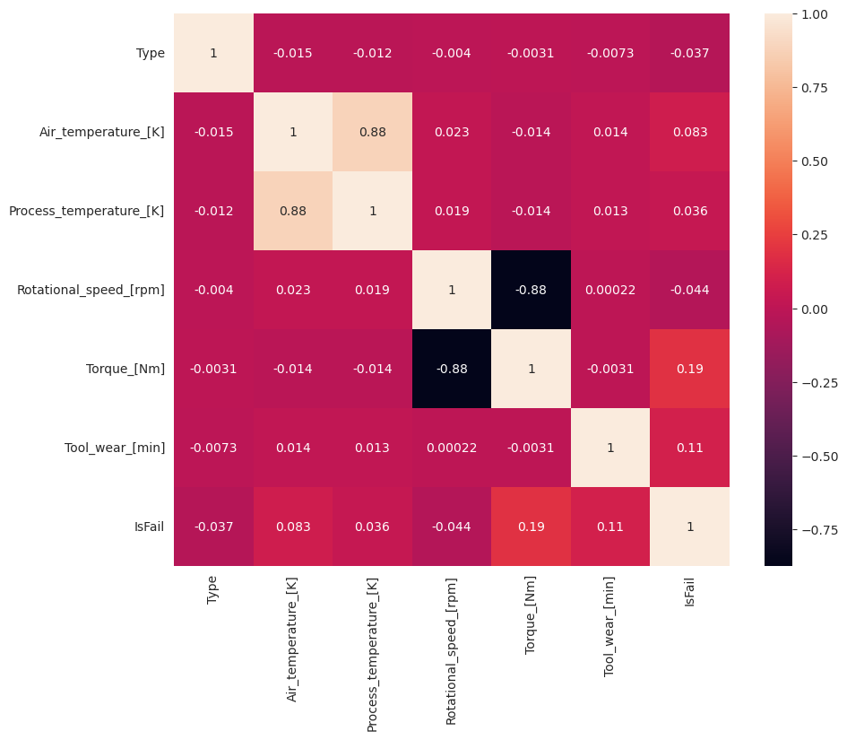
正如预期的那样,失败 (IsFail) 与所选特征(列)相关。 相关矩阵显示 Air_temperature、Process_temperature、Rotational_speed、Torque 和 Tool_wear 与 IsFail 变量的相关性最高。
# Plot histograms of select features
fig, axes = plt.subplots(2, 3, figsize=(18,10))
columns = ['Air_temperature_[K]', 'Process_temperature_[K]', 'Rotational_speed_[rpm]', 'Torque_[Nm]', 'Tool_wear_[min]']
data=df.copy()
for ind, item in enumerate (columns):
    column = columns[ind]
    df_column = data[column]
    df_column.hist(ax = axes[ind%2][ind//2], bins=32).set_title(item)
fig.supylabel('count')
fig.subplots_adjust(hspace=0.2)
fig.delaxes(axes[1,2])
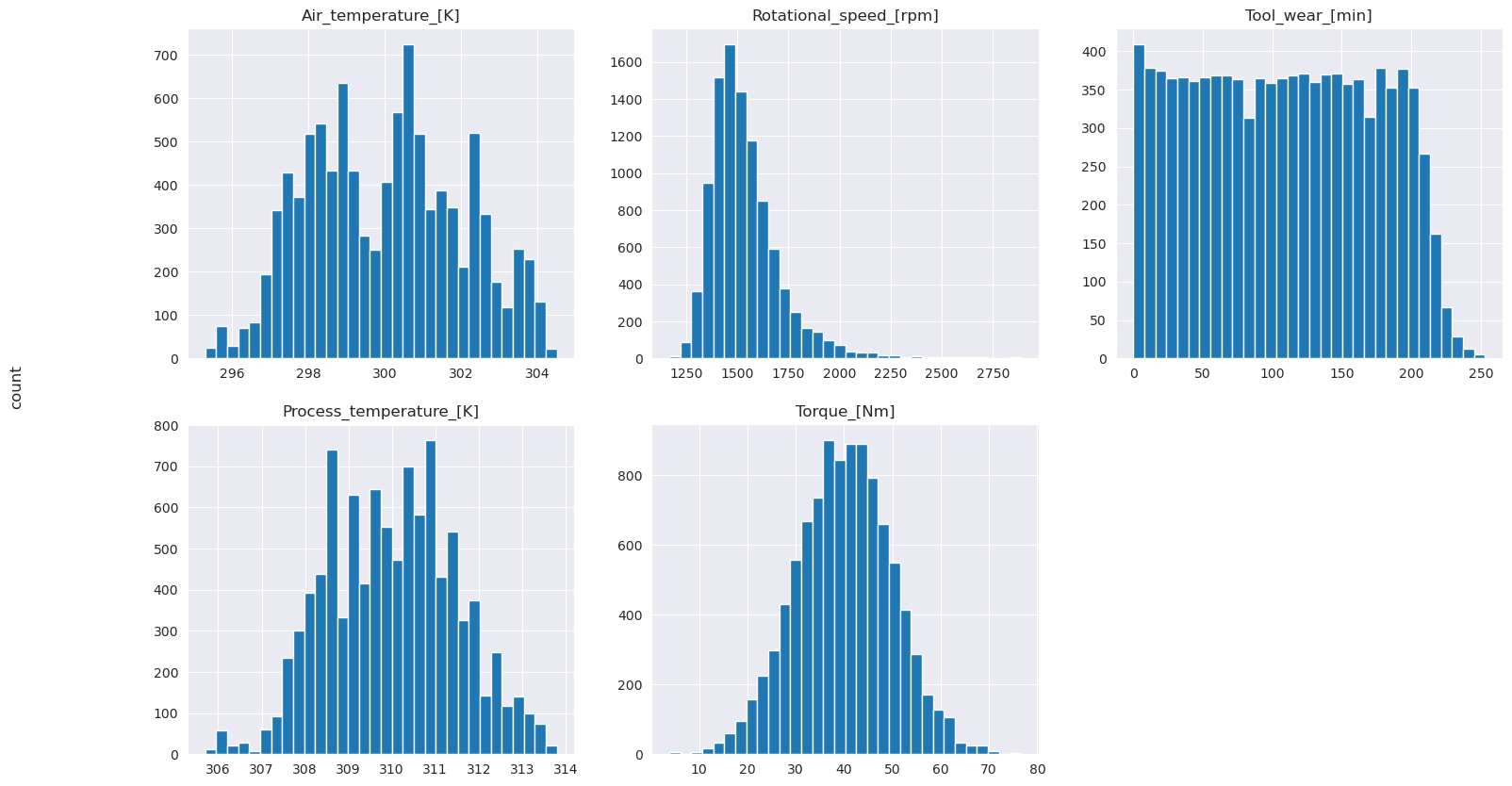
如绘制图表中所示,Air_temperature、Process_temperature、Rotational_speed、Torque 和 Tool_wear 变量并不稀疏。 它们似乎在特征空间中表现出良好的连续性。 这些绘图证实,在此数据集上训练机器学习模型可能会产生可靠的结果,可以推广到新数据集。
检查目标变量的类别不平衡
计算发生故障和未发生故障机器的样本数量,并检查每个类别的数据平衡(IsFail=0、IsFail=1):
# Plot the counts for no failure and each failure type
plt.figure(figsize=(12, 2))
ax = sns.countplot(x='Failure_Type', data=df)
for p in ax.patches:
    ax.annotate(f'{p.get_height()}', (p.get_x()+0.4, p.get_height()+50))

plt.show()

# Plot the counts for no failure versus the sum of all failure types
plt.figure(figsize=(4, 2))
ax = sns.countplot(x='IsFail', data=df)
for p in ax.patches:
    ax.annotate(f'{p.get_height()}', (p.get_x()+0.4, p.get_height()+50))

plt.show()
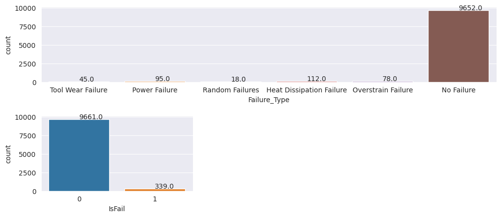
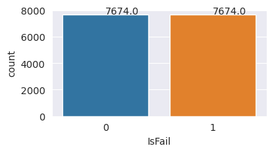
这些绘图表明无故障类别(在第二个绘图中显示为 IsFail=0)构成了大多数样本。 使用过采样技术创建更平衡的训练数据集:
# Separate features and target
features = df[['Type', 'Air_temperature_[K]', 'Process_temperature_[K]', 'Rotational_speed_[rpm]', 'Torque_[Nm]', 'Tool_wear_[min]']]
labels = df['IsFail']

# Split the dataset into the training and testing sets
from sklearn.model_selection import train_test_split
X_train, X_test, y_train, y_test = train_test_split(features, labels, test_size=0.2, random_state=42)

# Ignore warnings
import warnings
warnings.filterwarnings('ignore')
# Save test data to the lakehouse for use in future sections
table_name = "predictive_maintenance_test_data"
df_test_X = spark.createDataFrame(X_test)
df_test_X.write.mode("overwrite").format("delta").save(f"Tables/{table_name}")
print(f"Spark DataFrame saved to delta table: {table_name}")
过采样以平衡训练数据集中的类别
前面的分析表明数据集高度不平衡。 不平衡成为问题的原因在于,少数类的示例太少,模型无法有效了解决策边界。
SMOTE 可以解决问题。 SMOTE 这是一种广泛使用的过采样技术,可生成合成示例。 它以欧几里得距离为基础,根据数据点之间的距离生成少数类的示例。 此方法不同于随机过度采样,因为它创建的新示例不只复制少数类。 该方法可更有效地处理不平衡数据集。
# Disable MLflow autologging because you don't want to track SMOTE fitting
import mlflow

mlflow.autolog(disable=True)

from imblearn.combine import SMOTETomek
smt = SMOTETomek(random_state=SEED)
X_train_res, y_train_res = smt.fit_resample(X_train, y_train)

# Plot the counts for both classes
plt.figure(figsize=(4, 2))
ax = sns.countplot(x='IsFail', data=pd.DataFrame({'IsFail': y_train_res.values}))
for p in ax.patches:
    ax.annotate(f'{p.get_height()}', (p.get_x()+0.4, p.get_height()+50))

plt.show()
你已成功平衡数据集。 现在可以开始模型训练。
步骤 4:训练和评估模型
MLflow 用于注册模型、训练和比较各种模型,以及选取最佳模型进行预测。 可使用以下 3 个模型进行模型训练:
- 随机林分类器
- 逻辑回归分类器
- XGBoost 分类器
训练随机林分类器
import numpy as np
from sklearn.ensemble import RandomForestClassifier
from mlflow.models.signature import infer_signature
from sklearn.metrics import f1_score, accuracy_score, recall_score

mlflow.set_experiment("Machine_Failure_Classification")
mlflow.autolog(exclusive=False) # This is needed to override the preconfigured autologging behavior

with mlflow.start_run() as run:
    rfc_id = run.info.run_id
    print(f"run_id {rfc_id}, status: {run.info.status}")
    rfc = RandomForestClassifier(max_depth=5, n_estimators=50)
    rfc.fit(X_train_res, y_train_res)
    signature = infer_signature(X_train_res, y_train_res)

    mlflow.sklearn.log_model(
        rfc,
        "machine_failure_model_rf",
        signature=signature,
        registered_model_name="machine_failure_model_rf"
    )

    y_pred_train = rfc.predict(X_train)
    # Calculate the classification metrics for test data
    f1_train = f1_score(y_train, y_pred_train, average='weighted')
    accuracy_train = accuracy_score(y_train, y_pred_train)
    recall_train = recall_score(y_train, y_pred_train, average='weighted')

    # Log the classification metrics to MLflow
    mlflow.log_metric("f1_score_train", f1_train)
    mlflow.log_metric("accuracy_train", accuracy_train)
    mlflow.log_metric("recall_train", recall_train)

    # Print the run ID and the classification metrics
    print("F1 score_train:", f1_train)
    print("Accuracy_train:", accuracy_train)
    print("Recall_train:", recall_train)

    y_pred_test = rfc.predict(X_test)
    # Calculate the classification metrics for test data
    f1_test = f1_score(y_test, y_pred_test, average='weighted')
    accuracy_test = accuracy_score(y_test, y_pred_test)
    recall_test = recall_score(y_test, y_pred_test, average='weighted')

    # Log the classification metrics to MLflow
    mlflow.log_metric("f1_score_test", f1_test)
    mlflow.log_metric("accuracy_test", accuracy_test)
    mlflow.log_metric("recall_test", recall_test)

    # Print the classification metrics
    print("F1 score_test:", f1_test)
    print("Accuracy_test:", accuracy_test)
    print("Recall_test:", recall_test)
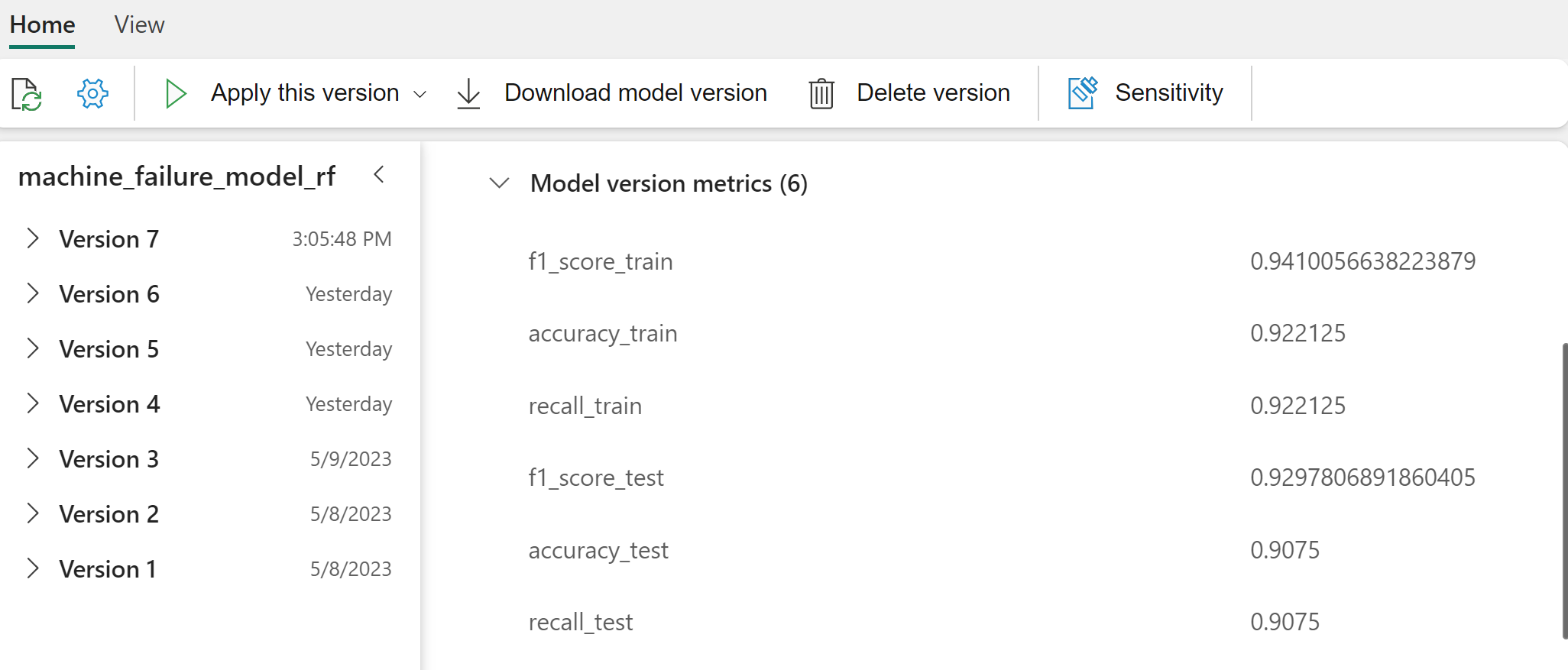
从输出来看,使用随机林分类器时,训练数据集和测试数据集都会产生约为 0.9 的 F1 分数、准确度和召回率。
训练逻辑回归分类器
from sklearn.linear_model import LogisticRegression

with mlflow.start_run() as run:
    lr_id = run.info.run_id
    print(f"run_id {lr_id}, status: {run.info.status}")
    lr = LogisticRegression(random_state=42)
    lr.fit(X_train_res, y_train_res)
    signature = infer_signature(X_train_res, y_train_res)

    mlflow.sklearn.log_model(
        lr,
        "machine_failure_model_lr",
        signature=signature,
        registered_model_name="machine_failure_model_lr"
    )

    y_pred_train = lr.predict(X_train)
    # Calculate the classification metrics for training data
    f1_train = f1_score(y_train, y_pred_train, average='weighted')
    accuracy_train = accuracy_score(y_train, y_pred_train)
    recall_train = recall_score(y_train, y_pred_train, average='weighted')

    # Log the classification metrics to MLflow
    mlflow.log_metric("f1_score_train", f1_train)
    mlflow.log_metric("accuracy_train", accuracy_train)
    mlflow.log_metric("recall_train", recall_train)

    # Print the run ID and the classification metrics
    print("F1 score_train:", f1_train)
    print("Accuracy_train:", accuracy_train)
    print("Recall_train:", recall_train)

    y_pred_test = lr.predict(X_test)
    # Calculate the classification metrics for test data
    f1_test = f1_score(y_test, y_pred_test, average='weighted')
    accuracy_test = accuracy_score(y_test, y_pred_test)
    recall_test = recall_score(y_test, y_pred_test, average='weighted')

    # Log the classification metrics to MLflow
    mlflow.log_metric("f1_score_test", f1_test)
    mlflow.log_metric("accuracy_test", accuracy_test)
    mlflow.log_metric("recall_test", recall_test)
训练 XGBoost 分类器
from xgboost import XGBClassifier

with mlflow.start_run() as run:
    xgb = XGBClassifier()
    xgb_id = run.info.run_id
    print(f"run_id {xgb_id}, status: {run.info.status}")
    xgb.fit(X_train_res.to_numpy(), y_train_res.to_numpy())
    signature = infer_signature(X_train_res, y_train_res)

    mlflow.xgboost.log_model(
        xgb,
        "machine_failure_model_xgb",
        signature=signature,
        registered_model_name="machine_failure_model_xgb"
    )

    y_pred_train = xgb.predict(X_train)
    # Calculate the classification metrics for training data
    f1_train = f1_score(y_train, y_pred_train, average='weighted')
    accuracy_train = accuracy_score(y_train, y_pred_train)
    recall_train = recall_score(y_train, y_pred_train, average='weighted')

    # Log the classification metrics to MLflow
    mlflow.log_metric("f1_score_train", f1_train)
    mlflow.log_metric("accuracy_train", accuracy_train)
    mlflow.log_metric("recall_train", recall_train)

    # Print the run ID and the classification metrics
    print("F1 score_train:", f1_train)
    print("Accuracy_train:", accuracy_train)
    print("Recall_train:", recall_train)

    y_pred_test = xgb.predict(X_test)
    # Calculate the classification metrics for test data
    f1_test = f1_score(y_test, y_pred_test, average='weighted')
    accuracy_test = accuracy_score(y_test, y_pred_test)
    recall_test = recall_score(y_test, y_pred_test, average='weighted')

    # Log the classification metrics to MLflow
    mlflow.log_metric("f1_score_test", f1_test)
    mlflow.log_metric("accuracy_test", accuracy_test)
    mlflow.log_metric("recall_test", recall_test)
步骤 5:选择最佳模型并预测输出
在上一部分,你训练了三种不同的分类器:随机林、逻辑回归和 XGBoost。 现在可以选择以编程方式访问结果,也可以使用用户界面 (UI)。
若要选择 UI 路径,请导航到工作区并筛选模型。
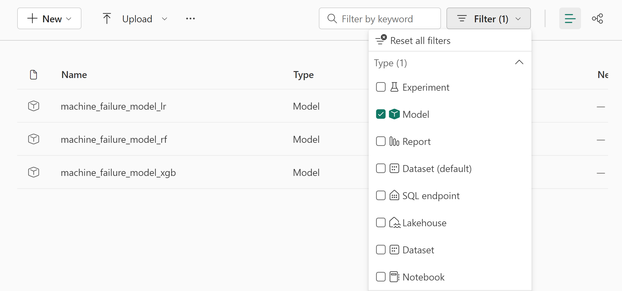
选择各个模型以了解模型性能的详细信息。
该示例演示了如何通过 MLflow 以编程方式访问模型:
runs = {'random forest classifier':   rfc_id,
        'logistic regression classifier': lr_id,
        'xgboost classifier': xgb_id}

# Create an empty DataFrame to hold the metrics
df_metrics = pd.DataFrame()

# Loop through the run IDs and retrieve the metrics for each run
for run_name, run_id in runs.items():
    metrics = mlflow.get_run(run_id).data.metrics
    metrics["run_name"] = run_name
    df_metrics = df_metrics.append(metrics, ignore_index=True)

# Print the DataFrame
print(df_metrics)
尽管 XGBoost 在训练集上获得了最好的结果,但它在测试数据集上的表现很差,这表明存在过度拟合。 性能不佳表示过度拟合。 逻辑回归分类器在训练和测试数据集上都表现不佳。 总体而言,随机林在训练性能和避免过度拟合之间取得了良好的平衡。
在下一部分中,选择已注册的随机林模型并使用 PREDICT 功能执行预测:
from synapse.ml.predict import MLFlowTransformer

model = MLFlowTransformer(
    inputCols=list(X_test.columns),
    outputCol='predictions',
    modelName='machine_failure_model_rf',
    modelVersion=1
)
使用创建的 MLFlowTransformer 对象来加载用于推理的模型,然后使用 Transformer API 在测试数据集上对模型进行评分:
predictions = model.transform(spark.createDataFrame(X_test))
predictions.show()
此表显示输出:
| 类型 | Air_temperature_[K] | Process_temperature_[K] | Rotational_speed_[rpm] | Torque_[Nm] | Tool_wear_[min] | 模型 |
|---|---|---|---|---|---|---|
| 0 | 300.6 | 309.7 | 1639.0 | 30.4 | 121.0 | 0 |
| 0 | 303.9 | 313.0 | 1551.0 | 36.8 | 140.0 | 0 |
| 1 | 299.1 | 308.6 | 1491.0 | 38.5 | 166.0 | 0 |
| 0 | 300.9 | 312.1 | 1359.0 | 51.7 | 146.0 | 1 |
| 0 | 303.7 | 312.6 | 1621.0 | 38.8 | 182.0 | 0 |
| 0 | 299.0 | 310.3 | 1868.0 | 24.0 | 221.0 | 1 |
| 2 | 297.8 | 307.5 | 1631.0 | 31.3 | 124.0 | 0 |
| 0 | 297.5 | 308.2 | 1327.0 | 56.5 | 189.0 | 1 |
| 0 | 301.3 | 310.3 | 1460.0 | 41.5 | 197.0 | 0 |
| 2 | 297.6 | 309.0 | 1413.0 | 40.2 | 51.0 | 0 |
| 1 | 300.9 | 309.4 | 1724.0 | 25.6 | 119.0 | 0 |
| 0 | 303.3 | 311.3 | 1389.0 | 53.9 | 39.0 | 0 |
| 0 | 298.4 | 307.9 | 1981.0 | 23.2 | 16.0 | 0 |
| 0 | 299.3 | 308.8 | 1636.0 | 29.9 | 201.0 | 0 |
| 1 | 298.1 | 309.2 | 1460.0 | 45.8 | 80.0 | 0 |
| 0 | 300.0 | 309.5 | 1728.0 | 26.0 | 37.0 | 0 |
| 2 | 299.0 | 308.7 | 1940.0 | 19.9 | 98.0 | 0 |
| 0 | 302.2 | 310.8 | 1383.0 | 46.9 | 45.0 | 0 |
| 0 | 300.2 | 309.2 | 1431.0 | 51.3 | 57.0 | 0 |
| 0 | 299.6 | 310.2 | 1468.0 | 48.0 | 9.0 | 0 |
将数据保存到湖屋中。 然后,数据可供以后使用,例如用于 Power BI 仪表板。
# Save test data to the lakehouse for use in the next section.
table_name = "predictive_maintenance_test_with_predictions"
predictions.write.mode("overwrite").format("delta").save(f"Tables/{table_name}")
print(f"Spark DataFrame saved to delta table: {table_name}")
步骤 6:在 Power BI 中通过可视化效果查看商业智能
使用 Power BI 仪表板以脱机格式显示结果。
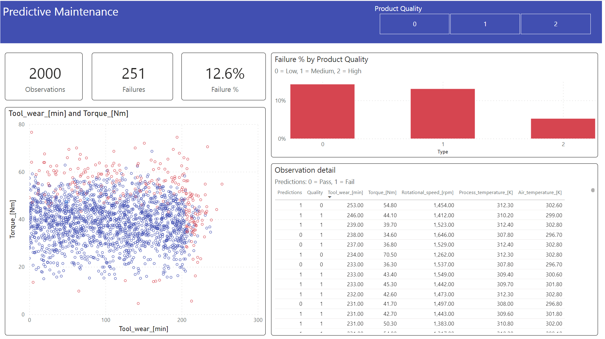
仪表板显示发生故障和未发生故障案例的 Tool_wear 和 Torque 之间存在明显区别,正如步骤 2 中早期相关分析所预期的那样。